Applications of Demand Supply Analysis (With Diagram)

The following points highlight the top six applications of demand supply analysis. The applications are: 1. An Excise or Per Unit Tax 2. A Sales Tax 3. A Production Subsidy 4. Import Tariffs 5. Export Subsidies 6. Controls on Prices and Quantities.

Application # 1. An Excise or Per Unit Tax:

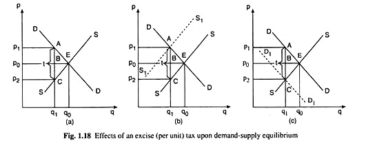
An excise or per unit tax is a fixed amount of tax, say, t, imposed on each unit of production of a commodity. The effect of a per unit tax of t on the market equilibrium of the commodity is illustrated with the help of Fig. 1.18.

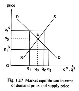
If such a tax is imposed, the sellers would shift the burden of the tax on to the buyers, so that, at the equilibrium quantity, we would have: the demand price of the buyers = the supply price of the sellers + the tax (t).

or, the demand price – supply price = t … (i)

or, the demand price = supply price + t … (ii)

or, the supply price = demand price −t … (iii)

Corresponding to (i), (ii) and (iii), it will have three ways depicted in Fig. 1.17 in which the effect of the imposition of a per unit tax on market equilibrium is illustrated. In all these figures, DD and SS are the demand and supply curves of the good, and p₀ and q₀ are the equilibrium price and quantity before the imposition of the tax that are obtained at the point of intersection E between the DD and SS curves.

According to (i), the equilibrium quantity, after the imposition of the tax, would be that q at which the difference between the demand price and supply price would be equal to t. This case has been illustrated in part (a) of Fig. 1.18. As it is known, at any q, demand price is obtained along the demand curve and the supply price is obtained along the supply curve.

Therefore, the new equilibrium q after the imposition of the tax would be one at which the vertical gap between the DD and SS curves would be equal to t. In Fig. 1.18(a), this equilibrium output has been obtained as q₁.

At q = q₁ the price including the tax that the buyers would have to pay is p₁₅ and the sellers, after deducting the tax from pi, would get a price of p₂ which is the supply price at q = q₁. At price p₁, the buyers are demanding the quantity q₁ and, at price p₂, the sellers are also supplying the quantity q₁, and so there is equilibrium and none of the buyers and sellers would tend to change the situation.

The second way of illustrating the effects of the imposition of a per unit tax upon the market equilibrium. According to (ii), at the post-tax equilibrium point, demand price would be equal to supply price +1.

Now, at any q, demand price would be obtained along the DD curve, but the supply price +1 would be obtained along a curve like S₁S₁ in Fig. 1.17(b) which is parallel to the SS curve but vertically above this curve by the distance t. The new post- tax equilibrium point would be obtained at the point of intersection A between the DD and S₁S₁ curves.

Here the equilibrium quantity would be qi and the price that the buyers would pay would be pi and the price that the sellers would receive would be p₂. In this situation, both the buyers and sellers would remain satisfied.

It is evident from the Figs. 1.17(a and b) that the post-tax equilibrium solutions are identical in both the cases—owing to the imposition of the tax, the equilibrium point would move from the point E to the point A.

Lastly, the third way of illustrating the effects of the imposition of a per unit tax has been shown in Fig. 1.17(c). According to (iii), at the post-tax equilibrium point, the supply price would be the (demand) price of the good minus the amount of tax (t).

That is why, in the figure, a curve D₁D₁ is drawn, which is parallel to DD but lies below the latter at a vertical gap equal to t. In this case, the post-tax equilibrium would be obtained at the point of intersection, C, between the D₁D₁ and SS curves.

This equilibrium solution would be the same as obtained in the previous two cases—here the equilibrium output is qi and the price (that the buyers pay) is pi and the sellers receive their desired price p₂. All are satisfied with this solution. The equilibrium point in this case would move from the point E to the point C.

If the post-tax equilibrium is compared with the pre-tax equilibrium, it is found that:

(i) After the imposition of the tax, equilibrium quantity bought and sold has decreased from q₀ to q₁.

(ii) The equilibrium price including the tax that the buyers would pay is p₁ which is greater than the pre­tax (equilibrium) price p₀, but not by the amount (t) of the tax.

(iii) Although the sellers have shifted the burden of the tax on to the buyers and although the buyers are paying a price which includes the tax, the entire burden of the tax, in fact, has not shifted to the buyers.

At the pre-tax equilibrium point, for both the buyers and sellers, the price was p = p₀. But, after the tax, the buyers are paying AB more as the price and the sellers are getting BC less as the price, AB + BC = AC being equal to t.

(iv) In respect of quantity also, the burden is shared—the buyers are buying less than before and the sellers are also selling less. Yet nobody is interested in any change and the equilibrium is there to stay.

Application # 2. A Sales Tax (Ad Valorem Tax):

A sales tax is an ad valorem (i.e., value-based) tax. It is imposed as a fixed percentage of the price of a commodity. Like the per unit excise tax, the sales tax also is collected from the buyer and paid to the government by the seller. The effects of a sales tax on market equilibrium can be illustrated in three ways (that are similar to the ways of illustration in the case of the excise tax).

It is continued to assume, for the sake of simplicity, that the demand and supply curves are straight lines.

Now, while illustrating the effects of a sales tax, any of the following three cases can be used:

At the equilibrium quantity−

demand price of the buyers − supply price of the sellers = the amount of tax (t) … (i)

or, the demand price = supply price + t … (ii)

or, the supply price = demand price -1 … (iii)

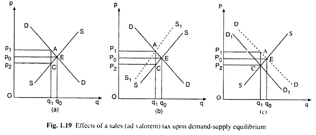
Here t is a variable, being a certain percentage of the supply price of the commodity—it is assumes that it is 20 per cent. The effects of a sales tax on the basis of (i) is explained with the help of Fig. 1.19(a). Here the pre-tax equilibrium point is E.

At this point or at q = q₀, the demand price and supply price are equal, both being equal to p₀. Now, (i) the post-tax equilibrium quantity the vertical gap between the DD and SS curves should be 20 per cent of the supply price.

In order to locate the new post-tax equilibrium quantity, move from the point E downward to left along the SS curve. Consequently, the vertical gap between the demand price and the supply price will increase. Eventually, stop at a point like C where the vertical gap between the DD and SS curves has been 20 per cent of the supply price (p₂).

At q = q₁ at point C, the market would be in equilibrium after the imposition of the tax. Here the sellers would get the price p₂, they would add the sales tax of 20 per cent of p₂ (= AC, say) to this price and would ask the buyer to pay the price p₁. At the price of p₁, the buyers would demand q₁ of output and at the price of p₂, the sellers would sell the same output (q₁), and so the market would be in equilibrium.

The impact of the imposition of a sales tax upon the market equilibrium is explained on the basis of (ii), and with the help of Fig. 1.19(b). Here DD and SS are the demand and supply curves for the good.

Initially, the equilibrium point is E (p₀, q₀). According to (ii), if a sales tax of 20 per cent is imposed, then at the post-tax equilibrium q, demand price would be equal to supply price plus a tax of 20 per cent of the supply price.

That is why, in Fig. 1.19(b), the S₁S₁ curve is drawn which gives us at any q, the supply price along the SS curve + a 20 per cent sales tax. Since, as q and the supply price increase, the amount of the tax (which is a certain percentage) will also increase, the vertical gap between the S₁S₁ and SS curves will increase.

Now, the post-tax equilibrium output, q₁, would be obtained at the point of intersection, A, of the DD and S₁S₁ curves. At this output, as per (ii), the demand price would be equal to the supply price + the tax. Here the buyer would pay a price of p₁ (including the tax) and demand q₁ of output and the sellers would obtain the price of p₂ and supply the same output. So the market would again be in a demand-supply equilibrium.

The demand-supply analysis in a third way to explain the effects of the imposition of a sales tax is also applied on the basis of (iii) and with the help of Fig. 1.19(c). Here as before, the DD and SS curves are the demand and supply curves of the good, and the pre-tax equilibrium point is E (p₀, q₀).

According to (iii), if the sales tax is imposed, then at the post-tax equilibrium q, the supply price would be the demand price—the amount of tax. That is why, in Fig. 1.19(c), a D₁D₁ curve is drawn which gives, at any q, the demand price minus the sales tax of a certain percentage (here 20 per cent) of the supply price. Since as q and the supply price increase, the amount of the tax also increases, and the vertical gap between the DD and D₁D₁ curves will increase.

Now, the post-tax equilibrium output, q₁, would be obtained at the point of intersection, C, of the D₁D₁ and the SS curves. At this output, according to (iii), the supply price (p₂) would be equal to the demand price (p₁) less the amount of the tax. Since at the price of p₁, the buyers would demand q, of output and at the price of p₂, the sellers would supply the same output, the market would again be in equilibrium.

The demand-supply equilibrium analysis can be applied to obtain the impact of a sales tax upon the equilibrium quantity bought and sold of the commod­ity concerned. It is presented in three ways of explaining the effect of the tax.

As is expected, the effects have been the same in all the three cases. A comparison between the pre­tax and post-tax equilibrium situations would take us to the same conclusions as it is ob­tained in the case of a per unit excise tax.

Application # 3. A Production Subsidy:

A production subsidy is granted by the government on a commodity to boost up its demand. It is collected by the producer of the commodity who charges the buyer a price which is lower than the supply price by the amount of subsidy.

The case of a production subsidy is similar in nature but opposite in effects if it is compares with a per unit excise tax or a sales tax. Suppose, a per unit subsidy of a fixed amount, S, is granted on a certain commodity, say, fertiliser. This means that the buyers would pay a price which would be smaller than the supply price by the amount ‘S’ i.e., here it would have

supply price – demand price = S … (i)

or, supply price = demand price + S … (ii)

or, demand price = supply price – S … (iii)

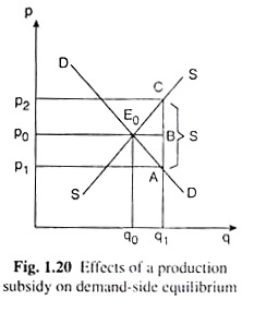
The effects of a subsidy upon the equilibrium price and quantity is explained on the basis of (i) above, with the help of Fig. 1.20, which is similar to Fig. 1.18(a). The effects of a per unit subsidy may also be explained on the basis of (ii) and (iii) in a similar way as those of a per unit

In Fig. 1.20, DD and SS are the demand and supply curves for the commodity, and the initial equilibrium point is E (p₀, q₀). However, after the grant of the subsidy, the equilibrium quantity would be one at which the demand price would be smaller than the supply price by the amount of subsidy, S.

That is why, in order to find this equilibrium quantity, move along the DD curve from the point E downward towards right till the vertical gap between the SS and the DD curves becomes equal to S.

Therefore, the equilibrium quantity after subsidy would be one like q₁ at which the said vertical gap is AC = S. At q = q₁, the sellers would get the price of p₂ and the buyers would pay the price of p₁, p₂ – p₁ being equal to S. At the price of p₁, the buyers would demand the quantity q, and at the price of p₂, the sellers would sell the same quantity. So the market would be in equilibrium at q = q₁.

If  the post-subsidy equilibrium is compared with the pre- subsidy situation, it would be found:

(a) After the grant of sub­sidy, equilibrium q has increased from q₀ to q₁ whereas in the case of per unit excise tax, q decreases from q₀ to q₁.

(b) The equilibrium price for the buyers is p₁ which is less than the equilibrium price of the sellers by the per unit subsidy, S. But in the case of a per unit tax the buyers’ equilibrium price is greater than the sellers’ price.

(c) Although the buyers are getting a subsidy of S per unit, the post-subsidy equilibrium price for them is not less than the pre-subsidy equilibrium price by the amount of the subsidy, AC = S, but by a smaller amount, AB. On the other hand, the sellers are also getting a benefit of price rise—their price rises by BC. It may be noted that AB + BC = AC = S.

(d) In respect of quantity also, both the buyers are sellers are sharing the benefit of subsidy the buyers are buying more and the sellers are also selling more. In the case of the per unit tax or sales tax, the buyers buy less and the sellers also sell less.

The case of a per unit subsidy. Subsidy may also be given as a percentage of the supply price. The effects of a percentage subsidy may be explained in a similar way as those of a percentage sales tax. The students may work out this explanation as an exercise.

Application # 4. Import Tariffs:

Tariffs are taxes that are imposed on the articles that cross the borders of a country—either come into the country or go out of it. Therefore, tariffs may be import tariff or export tariff. Import tariffs are more commonplace.

They are imposed by almost all the countries. Develop­ing countries impose tariffs on the articles to be imported with a view to protecting domestic industries and employment. The simple demand-supply analysis may be used to explain the effects of an import tariff.

Suppose, a good domestically produced and consumed by a country, is also traded in the perfectly competitive world market where the price of the good is, say, p_f. In the absence of any tariff, the producers and consumers within the country can sell and buy any quantity of the good at this price.

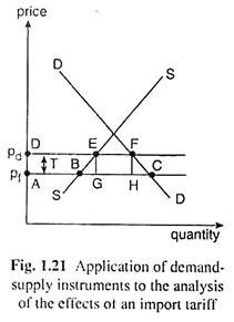
In Fig. 1.21, the demand curve and the supply curve of the good within the country are DD and SS, respectively. At the price of p_f, demand for the good is AC and its supply is AB. Therefore, within the country, there is an excess demand for the good of the amount BC. In order to satisfy the excess demand, the country would have to import this amount, i.e., BC.

Now, with a view to reducing the quantity of the good to be imported, the country imposes an import tariff of, say, T per unit. Then, within the country, the price of the good would in­crease. It would be, say, p_d where p_d = p_f + T.

At the higher price, p_d, demand for the good would diminish and the supply of the good increase within the country, reducing the excess demand gap from BC to EF. That is, the quantity of the good to be imported would reduce from BC to EF. Here the government would collect a revenue at the rate of T per unit of imports, the total revenue being given by EF x T = □ EFHG.

The government of a developing country often imposes import tariff with view to protect production and employment within the country. However, the imposition of an import tariff may be construed as imposition of restrictions on international trade.

That is why, sometimes, instead of imposing an import tariff, the government may decide to provide the domestic producers with a subsidy at the rate of T per unit of the good produced. As a result, the price received by the producers would be p_f + T = p_d whereas the consumers would still pay the price p_f.

Hence, the quantity produced and supplied of the good would rise to DE from AB. But, since the consumers would still be paying what they had been initially, i.e., the price p_f, the quantity demanded would remain unchanged at AC.

Since supply has increased and demand has remained unchanged, the quantity to be imported will fall, but not by as much as in the case of imposition of tariff. The quantity of imports now would be GC, EF < GC < BC.

However, in order to avoid the imposition of an import tariff, if the government gives a subsidy to the producers at the rate of T and, at the same time, imposes a consumption tax of T per unit, then the producers will receive the price p_d = p_f + T and, at the same time, the consum­ers would pay a price p_d = p_f+ T. As is evident, this case is very much similar to the imposition of an import tariff.

For here also, the domestic supply will increase from AB to DE and the domestic demand will fall from AC to DF. As a result, the quantity to be imported would fall from BC in the initial situation to EF in the current situation.

On the revenue side, the government now collects a revenue of DF x T = □ ADFH from the consumption tax, but pays a total amount of subsidy to the producers equal to DE x T = □ ADEG. Therefore, the government’s net revenue from subsidy-and-tax case would be equal to □ ADFH − □ ADEG = □ EFHG which is the same as the revenue the government earned from the imposition of import tariff at the rate of T.

Ttherefore, It is concluded that an import tariff of T per unit has exactly the same ef­fects as a production subsidy at the rate of T along with a consumptions tax of T per unit. From this it is clear that it is the consumers who actually pay the cost of a tariff on the imports of a good.

Application # 5. Export Subsidies:

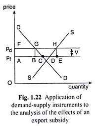
The countries, in order to augment their exports, give subsidy to the exports of different items so that their producers might successfully compete in the world market. The demand-supply analysis may be used to explain the effects of an export subsidy. Let us suppose, in Fig. 1.22, DD and SS are the domestic demand and supply curves of a good.

Suppose, without any tariff or subsidy the domestic price of the good is p_f which is actually the ruling price in the competitive world market. At this price, the quantities demanded and supplied of the good within the country is AC and AD, and the supply quantity being greater than the demand quantity, their difference, CD, is exported.

Suppose, the government, with a view to stimulating exports, introduces an export subsidy of V per unit of exports. As a result, the produc­ers of the good would enhance its domestic price, since they will be receiving the price inclusive of the subsidy for what­ever quantity they might export.

The price now would be p_d = p_f + V. As price rises, demand for the good would fall to FG and supply would rise to FH, and so the export gap now would be GH which is larger than what it was initially, i.e., CD. The cost to the government on account of exports subsidy is GH x V = □ GBEH.

The effect would be the same if the government gives a production subsidy of V per unit of pro­duction and, at the same time, imposes a consumption tax of V per unit. Then also the producers will receive the price p_d – p_f + V and the consumers will pay a price p_d = p, + V.

Consequently, demand for the good will fall to FG and supply will rise to FH, and so the export gap will be GH. The production subsidy now would cost the government an amount equal to FH x V or □ AFHE while the consumption tax would give the government a revenue equal to FG x V or □ AFGB.

Therefore, the net cost to the government of the tax-subsidy combine would be □ AFHE − □ AFGB = □ GBEH which is the same as the cost to the government of the export subsidy. It follows then that an export subsidy is equivalent to a production subsidy plus a consumption tax.

In the above analysis, for the sake of driving home the main point in a simple manner, it is assumed away the costs of tax collection and disbursal of subsidies.

Application # 6. Controls on Prices and Quantities:

How the demand-supply analysis may be used to explain the government policies that are undertaken:

(i) To prevent prices from rising to their market equilibrium levels,

(ii) To prevent prices from falling to their market equilibrium levels, and

(iii) To prevent quanti­ties from reaching their market equilibrium levels.

(i) Sometimes the equilibrium level of the price of an essential commodity may become so high that the low-in­come consumers would not be able to buy it. In such a case, the government price control measures may try to prevent the price from reaching the height of the equilibrium level.

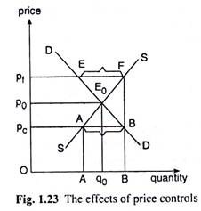
The point is explained with the help of Fig. 1.23 where the DD and SS curves are the demand and supply curves for the commodity, and p₀ and q₀ are the equilibrium price and quantity.

Now, if the equilibrium price of p₀ appears to be too high for the low-income consumers to enter the market, the gov­ernment may undertake a policy of imposing a ceiling price. For example, the government may declare that the price of the commodity must not be greater than p_c.

But the implementation of this policy would not be without problems. For, as the ceiling price is imposed (below the equilibrium price), the supply of the good would fall below the equilibrium quantity of q₀ and the demand would rise above the equilibrium quantity.

Thus, a shortage would develop in the market, demand being greater than supply. In Fig. 1.23, the amount of this shortage has been AB. If this shortage persists, there would develop a black market of the commodity and the government’s purpose would be frustrated. To solve the problem of excess demand, the gov­ernment may introduce a system of rationing.

This means, at the controlled price which is smaller than the market equilibrium price, the buyers would not be able to buy any amount that they wish to buy. Rather, they would have to be satisfied with the rationed quantity they are allotted.

Of course, black market may not develop in the case of imposition of price ceiling on each and every commodity. For example, in the case of price controls on natural gas, the excess demand may get transformed into the demand for alternative fuels, e.g., heating oil, electricity, or coal.

Similarly, in the case of rent controls, the excess demand may go into alternative housing arrangements.

One of the major objectives of the controls on natural gas prices, rent controls, etc. is to prevent large income transfers to the owners of these resources. What condi­tions such transfers may be prevented.

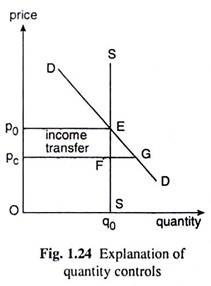
It is considered in the case where the quantity supplied is given and constant-it is equal to, say, q₀ in Fig. 1.24, giving us a vertical supply curve SS of the commodity. Here DD is the demand curve. The equilibrium price is p₀ and the equilibrium quantity can be nothing but q₀ = constant.

Suppose, the ceiling price that is imposed is p_c < p₀. Although the price has been fixed on a lower level, the quantity supplied cannot fall since it is fixed at q₀. The quantity demanded, however, rises by FG creating an excess demand of the same amount.

The excess demand, however, will remain unsatisfied, for, by no means, supply can be increased. Initially, at p = p₀ and q = q₀, the buy­ers were spending an amount equal to □ Op₀Eq₀. But after the price control, at p = p_c and q = q₀, they are spending an amount equal to □ Op_cFq₀.

So after the control has been imposed, the buyers’ expenditure has decreased by the amount equal to □ p₀EFp_c. In other words, by means of price control, the government has been able to transfer an amount equal to □ p₀EFp_c from the producers or resource-owners to the buyers.

In case of rent controls, if it assumes that the quantity of housing is fixed at q₀ in Fig. 1.24, then the price control would result in an income transfer from the landlords to the tenants who are currently occupying the apartments or houses.

But, as rent is fixed on a lower level, some new consumers would enter the market for apartment leasing. But, since the supply is fixed, their demand, i.e., the excess demand, would remain unsatisfied, i.e., they cannot obtain any rental housing in the market.

Similarly, in the market for natural gas, the price control would result in income transfer from the natural gas producers to the consumers. Here also the excess demand from the exist­ing or new customers cannot be satisfied.

(ii) So far as it is discussed price control by the imposition of ceiling (or, maximum) price. The imposition of floor (or minimum) price. The government undertakes such a policy when the equilibrium price in the market is considered to be too low for the sellers of a good or service to produce and sell it with a reasonable amount of profit.

For example, the market equilibrium prices of some agricultural goods are sometimes found to be so low that the government cannot but undertake price support programmes for them.

In Fig. 1.23, the demand and supply curves for a good are given to be DD and SS and the equilibrium price and quantity in the market have been p₀ and q₀, respectively. Now, if this price is considered too low for the producers, then the government would have to set a floor or minimum price for the good above its equilibrium price.

Suppose, this price is p_f > p₀. At p = p_f > p₀, quantity supplied will be more than q₀ and the quantity demanded would be less than q₀. As a result, there will be an excess supply in the market of the amount EF.

The problem of excess supply in this case can be resolved if the government is ready to purchase the whole of excess supply at the controlled price from the farmers; or the government may purchase a part of the excess supply and subsidies the farmers in storing the remaining part.

The concept of floor price may also be applied to case of wage determination. Sometimes the price of some particular type of labour may be so low in the market that the concerned workers would have to live below the subsistence level.

In such a case, the government would have to go in for enacting a minimum wage legislation stipulating that the price of labour (wage) of the concerned workers must not fall below a minimum level, like p_f in Fig. 1.23, although the equilibrium wage is a bit lower, like p₀. Since p_f is higher than the demand-supply equilibrium price (wage rate) p₀, there would occur an excess supply in the labour market.

In the case of minimum wage legislation, the excess supply of labour may go into a pool of unemployed. Subsequently, they may be given unemployment insurance benefits or they may get jobs that are not covered by minimum wage legislation.

(iii) Let us now come to the case of quantity controls. An example of quantity control is an import quota. An import quota is a direct quantitative restriction on the amount of a particular item of imports of a country.

The effect of an import quota is the same as that of an import tariff that is discussed with the help of Fig. 1.21. In this figure, if there is no tariff or control of any sort, then at the price p_f, the quantity that would have to be imported is BC.

But if the government wants to restrict the quantity of imports to EF = GH, then at p = p_f, only the amount GH or EF out of the excess demand BC would be satisfied, and the amount BG + CH cannot be satisfied. Therefore, the price would rise till it becomes p = p_d. For, at this price, the amount of excess demand is EF which the government has decided to import.

Now, the govern­ment may restrict imports by issuing import licenses equal to the amount EF. The licenses may be issued by lottery or by auction. In the former case, the lucky importer would import the good at the price p_f but sell it at the price p_d = p_f + T.

Therefore, the importers together would reap a benefit equal to EF x T = □ EGHF. In the latter case, i.e., in the case of auction, the government would be able to sell the licenses at a price that would give it a revenue equal to □ EGHF.

The case of a per unit tax that is explained with the help of Fig. 1.18(a), is also a case of quantity control. This is comparable to the case where the government does not allow the quantity produced to be as high as q₀ which is the market equilibrium quantity, instead, it restricts the quantity of output to q₁₍ (q₁ < q₀), by issuing production licenses for that amount.

Here also, if the licenses are issued by means of lottery, then the lucky producers who get the licenses would sell the amount at p = p₁ although they were willing to sell at p = p₂. Thus, they would be able to earn profits of the amount (p₁ – p₂)q₁.

But if the licenses are auctioned off, then the government would be able to get the revenue of the amount (p₁ – p₂)q₁ which is exactly the same as the revenue it could earn from a per unit tax. It is seen that the import quota restrictions and the restrictions implemented by means of a per unit tax are similar.