Keynesian Theory of Income and Employment

In this article we will discuss about the Keynesian Theory of Income and Employment.

Keynes’s Concept:

1. The level of employment is directly related to the level of production or output (Y).

2. In a market economy, planned spending on busi­ness output will determine the level of produc­tion. Businesses adjust their levels of production to accommodate demand for their products. Put simply, “Supply adjusts to demand.” Contrast this statement with Say’s Law, which said, “Sup­ply creates its own demand.”

3. Since employment depends on production and production responds to spending, the level of em­ployment in a market economy depends on the level of planned spending in the economy.

In fact, Keynes turned the order around from the classical model. In the classical model, the labour market determined the level of output and therefore, the position of the vertical aggregate supply curve.

In the Keynesian model, since there are unemployed resources, the aggregate supply curve will be hori­zontal, not vertical. Aggregate demand determines the level of output, and the level of output determines the level of employment. Aggregate demand, which only determined the price level in the classical model, now has the starring role: determining the level of real output.

According to Keynes, while consumption has an induced, or endogenous, component, invest­ment is an autonomous, or exogenous component of aggregate desired expenditure. These two functions are known as the building blocks of the theory of income determina­tion (as presented by Keynes).

On the basis of these two functions we may now see how the equilibrium level (size) of national income is determined. Just as the behaviour of prices and quantities in individual markets can be explained by the interaction of de­mand and supplies, the behaviour of a country’s total output (or its national income) depends on the econ­omy’s total demand and total supply.

The modern theory of income determination was presented in 1936 by J. M. Keynes, the great English economist. In this theory he stressed the influence of total demand in explaining the short-term behaviour of national income.

Fundamental Assumptions:

Following Keynes, we make the following two fundamental assumptions:

1. The potential output of an economy is noth­ing other than its full employment output (national income). This is the maximum output the economy is capable of producing by utilizing all its existing resources of land, labour power, capital and organi­zation.

2. Business firms (or producing units) will pro­duce as much output as is necessary to satisfy the existing level of demand at current prices. Output ex­pansion will continue until full employment is reach­ed. The implication is clear: as long as there is sur­plus capacity there is no need for prices to rise so as to stimulate production.

If we make these two assumptions we observe that the economy’s GNP or national income depends on aggregate demand (i.e., consumption demand and investment demand).

If demand is so strong as to absorb the full employment GNP of the economy, the economy’s actual output will be equal to its potential, i.e., maximum capacity output. If, on the other hand, there is enough demand to buy just 80 per cent of the economy’s potential output, then actual output will exactly be 80 per cent of full-employment GNP.

Basic Concept of Equilibrium National Income:

Since equilibrium refers to a position of rest or balance, national income is said to be in equilibrium when it remains unchanged at a particular level, i.e., when there is no tendency for it either to rise or to fall. The level of national income thus achieved is treated as the equilibrium national income. (When national income moves up or down we speak of a state of disequilibrium).

Equilibrium Conditions:

There are two alternative ways of stating the equi­librium conditions for national income:

1. Desired expenditure equals actual output (the income-expenditure approach).

2. Saving equals investment (the leakages-injections approach).

Both the approaches give the same result. But each has different insights. Thus, it is useful to study both.

The Income-Expenditure Approach:

The income-expenditure approach is illustrated in Table 34.1. It is quite obvious that in a modern economy using money as a medium of exchange all income is generated by production, i.e., the entire na­tional income is paid out to households, so that the income of the households is exactly equal to the value of output i.e., GNP or GNI.

The Relation between Income and Expenditure:

It is necessary to consider, at the beginning of our analysis, how much expenditure is planned at each level of national income. Let us assume that business firms are producing an output of Rs. 1600 crores. In­come of the household sector is also Rs. 1600 crores. But, according to Table 34.1 total planned expenditure of households and firm on C and I is Rs. 1800 crores at that level of income.

If firms continue to produce their current output level of Rs. 1600 crores when planned expenditure is Rs. 1800 crores, one of the following two things must happen: either (1) production plans will be fulfilled and expenditure plans unfulfilled or (2) expenditure plans will be fulfilled and production plans will be unfulfilled. We may now consider each of these extreme possibilities in greater detail.

Unfulfilled expenditure plans:

Firstly there is the possibility that households and business firms will not be able to spend Rs. 200 crores in excess of the value of current output that they plan to spend.

There will be excess demand for commodities and shortages will appear in the market(s). These will provide sig­nals to the firms to increase their output so as to meet the excess demand by selling more. As and when they do this, national income rises.

Unplanned changes in stocks:

Business firms of­ten hold stocks of finished goods because production and sales do not always coincide. So the second pos­sibility here is that households and firms will be able to fulfil their expenditure (consumption and invest­ment) plans by purchasing goods that were produced in the past and held in stock.

Since supply = produc­tion ± stocks, the only way to fulfil consumption and investment plans in this case is by purchasing exist­ing stocks of goods.

Thus, in our example, the stocks of business firms must fall by Rs. 200 crores in or­der to meet excess demand of the same amount. It is because the desired expenditure of the community of Rs. 1800 crores is greater than the current output of Rs. 1600 crores by exactly Rs. 200 crores.

This situ­ation will continue as long as stocks last, with more goods being sold than are currently being produced. However, stocks will get exhausted sooner or later.

But firms will adopt necessary measures to meet the extra demand well in advance. The additional output will then permit business firms to sell more without a further reduction of stocks. As production increases the demand for factors will increase and the factor- owners will receive extra income.

Thus, in both the case (i.e., case of unfulfilled expenditure plan and un­planned changes in stocks) the effect of an excess of planned expenditure over actual output is a rise in GNP or in national income.

In each of the two cases described above the following conclusion will hold at any level of national income or national output at which total planned (desired) expenditure exceeds total output, national income will have to rise—sooner or later.

Let us go back to Table 34.1 for the sake of il­lustration. Assume that national income is Rs. 3,200 crores. When income reaches this level, the total ex­penditure of households and business firms on con­sumption and investment goods is Rs. 3,000 crores. If firms continue to produce a total output of Rs. 3,200 crores there will be undesired inventory of Rs. 200 crores, i.e., Rs. 200 crores worth of goods will remain unsold.

This will lead to a rise in the level of stocks of business firms. But this is not desirable for obvi­ous reasons. Firms will, therefore, not permit their stocks to increase continuously.

If they are forced to hold stocks of finished goods due to low demand, a cutback in production is inevitable. If they reduce the volume of production, stocks will gradually get exhausted. Consequently output will be equal to cur­rent sales, sooner or later.

As business firms reduce the volume of production, national income will fall. Thus, it is quite clear that at any level of national in­come for which total desired (planned) expenditure falls short of total output (GNP), national output or national income will sooner or later fall.

Equilibrium Income:

Suppose, now national income is Rs. 2,400 crores in Table 34.1. At this level, and only at this level, to­tal planned expenditure of households and business firms is exactly equal to the amount of output pro­duced or income generated by the economy (i.e., to­tal planned expenditure is equal to national income). Households are just able to buy what they wish to without causing stocks to rise or fall.

Business firms are just able to sell their entire current output, with­out adding to or subtracting from their stocks.

Since current output is just sufficient to meet current de­mand there is hardly any incentive for firms to pro­duce more or less. Thus national income remains un­changed. Since there is neither excess demand nor ex­cess supply there is no upward or downward pressure on national income either.

When national income re­mains unchanged at a particular level without either increase or fall it is said to be in equilibrium. Thus, national income reaches its equilibrium level only when ag­gregate planned expenditure (C + I) is exactly equal to current total output.

The income-expenditure approach may now be illustrated diagrammatically. In Fig. 34.1 the aggre­gate expenditure function is E. It is the sum-total of C and I. And is obtained by plotting column (iv) Table 34.1. The 45° line is called the income line (or guideline) because it shows different levels of income.

It is obtained by plotting column (i) of Table 34.1. Na­tional income reaches equilibrium at point A where desired expenditure is equal to national income (out­put). What is the logic of this equilibrium? Below the equilibrium level of income, the E line lies above the 45° line (labelled E = Y). This shows that total planned expenditure exceeds national income.

When people want to buy more goods than is being pro­duced there will be a pressure on national income to rise, as is indicated by the arrow to the left of point A. On the other hand, above the equilibrium level of income, the E lie above the income line.

This shows that planned expenditure is less than income. What people express their desire to buy less than what the economy is currently producing, there is a pressure on national income to fall, as is indicated by the arrow to the right of point A.

Equilibrium is reached at the level of income Y_e where the total expenditure line, E, cuts the income line (or the 45° line). At this level of income de­sired expenditure, shown on the vertical axis, it ex­actly equal to actual national income, shown on the horizontal axis.

From Table 34.1 one thing is quite clear: there is always a tendency for national income to move to­wards its equilibrium value. The reason is easy to find out: aggregate desired expenditure is greater than na­tional income where income is below its equilibrium value, and less than national income when income is above its equilibrium value.

Only when aggregate planned expenditure is exactly equal to current na­tional income (output) expenditure plans are exactly matched by output. People wish to buy an amount equal to the value of what is produced. Since peo­ple, plan to buy exactly what is produced, there is no tendency for national output (GNP) or income to rise or fall. National Income remains unchanged and is said to be in equilibrium.

This is the essence of the Keynesian theory of income (output) determination. Since income is the result of employment of resources, including manpower, this theory is also known as the Keynesian theory of income and employment.

Planned and Actual Expenditure:

It was Keynes who first discovered the relation between planned and actual figures. So it is necessary to refer to the relation between output and planned expenditure on one hand and actual expenditure on the other hand.

A study of national income account­ing (estimation) shows that as a matter of definition, the value of the nation’s output or GNP is equal to actual expenditure on that output and to actual factor incomes generated by producing that output. These are just three different ways of looking at the same figure, the money value of total output produced.

But what is relevant for Keynesian theory of in­come determination is planned or desired expendi­ture. We have seen above that an inequality (or imbal­ance) between planned expenditure and total output creates disequilibrium in a simple two-sector econ­omy.

There is no reason why the planned expenditure of households and firms on consumption and capital goods should always be equal to the value of total output of such goods. In fact, we have observed that when these two magnitudes are not the same, national income must rise or fall.

We have also noted that when planned expen­diture is equal to total output, national income is in equilibrium. Keynes’ income-expenditure approach determines the equilibrium level (value) of national income at that point. The implication is very simple: in a private two-sector economy people wish to buy the total output that firms succeed in producing.

The Leakages-Injections (Saving-Investment) Approach:

The circular flow of income that is studied in macroeconomics is defined as the flow of payments from households to business firms (to pay for con­sumption goods) and from firms to households (to pay for factor services in the form of rent, wages, in­terest, profits and dividends).

The Basic Concept of Leakages and Injections:

It is to be noted, at the outset, that there are both injections into and leakages from the circular flow of income. An injection or an addition refers to pay­ments received by firms or households that are not derived from the spending of the other group. Op­positely, a leakage or a subtraction (or withdrawal) refers to payments received by firms or households that are not passed on through their current expendi­ture.

In a different language, an injection is an income receipt that did not arise from household spending while a leakage is that portion of an income receipt which does not lead to further spending (or responding). As R. G. Lipsey and Colin Harbury have rightly put it: “Leakages are identified by looking forward to see where income goes, while injections are iden­tified by looking backwards to see where the income came from.” In the simple two-sector economy we are considering now investment is the only injection and saving is the only leakage. We now explain the reason(s).

Saving as a Leakage:

In all non-socialist countries the major portion of saving originates from the household sector. Here we assume that all saving is household saving. (This means that business firms do not retain any dividend for reinvestment. They distribute their entire after-tax profits as dividends).

Household saving is income received by house­holds and not passed on to firms through extra con­sumption spending. To the extent households save they reduce their expenditure on consumption goods.

The amount that is saved is not passed on to business firms in the form of sales receipts. So the demand for their products falls. They are forced to cut back production. As a result national income falls. Hence saving is called a leakage from the circular flow of income.

Let us consider an extreme situation. Suppose households save their entire income and spend noth­ing on consumption goods. Thus the entire income received by the household sector leaks out of the cir­cular flow; none of it is passed on to firms through spending on consumption goods.

Since there is no spending firms will receive no income. Being unable to sell anything they will gradually reduce their out­put of consumption goods to zero. Thus we reaffirm the statement that saving is a leakage.

Investment as an Injection:

If a firm makes investment the income of firms producing investment (capital) goods rises. If a tex­tile producing company places more orders for tex­tile producing machines the industry manufacturing such machines will get more orders.

Thus an act of investment leads to an increase in income of firms that produce capital goods such as plant, equipment and machinery. Since investment spending creates income, investment represents an injection of income into the circular flow.

The Relation between Saving and Investment:

Saving is the supply of capital and investment is the demand for capital. Some people save and others invest. Saving is mainly done by households but in­vestment activities are largely carried out by business firms.

Moreover, the motives for saving and invest­ment are different. While households save for cer­tain personal reasons business firms invest for mak­ing profits. Thus a divergence between saving and investment is a logical possibility.

It is quite possible for business firms to plan to increase their investment spending at a time when households are planning to reduce their saving (in order to increase consump­tion). It is also possible for firms to plan to reduce their investment expenditure at the same time that households plan to increase their saving.

No doubt financial institutions like banks help to channel sav­ings into investment. But since saving and investment decisions are taken by two different groups of people the planned saving of households are unlikely to be equal to the planned investment of business firms.

Saving and Investment in the Circular Flow Dia­gram:

Figure 34.2 presents a circular flow diagram. It shows two types of flows with expenditure flows go­ing from firms to households (as income payments) and from households to firms (through consumption purchases). Since saving is a leakage it is marked with a minus sign.

Likewise since investment is an injection it is marked with a plus sign. Financial in­stitutions operating in the capital market act as a link between households and business firms.

Since house­holds decide on the flow of the leakages that they wish to make in the form of saving, while firms decide on the flow of injections that they wish to make in the form of investment, the flow of planned saving need not necessarily be equal to the flow of planned invest­ment at a fixed point of time.

The Influence of Saving and Investment:

Since saving is that portion of income of a house­hold which is not passed on by way of further spend­ing, it exerts a contractionary influence on the circular flow of income. It reduces the flow of income.

Investment, on the other hand, is revenue re­ceived by firms that does not arise out of household’s consumption spending. In the case of investment goods we see that business firms are both buyers and sellers. The firms which produce and sell capital (in­vestment) goods like machines have to employ factors of production. The owners and suppliers of the fac­tors are largely the households.

Thus, an increase in the demand for factors, in the capital goods produc­ing industries, creates income of the household sector. A portion of such income is spent by households on consumption goods like food, clothing, etc. produced by firms. The firms producing and selling such goods get extra revenue.

Thus, investment increases the flow of income and is therefore rightly called an injection.

Equilibrium Income:

In view of the above argument it is quite obvious that the circular flow is in equilibrium with national income remaining steady—when the volume of leak­ages (caused by saving) is equal to the volume of injec­tions (caused by investment). We may now examine how this happens.

To see how national income equilibrium is achie­ved through saving and investment we look at Table 34.2. Let us first consider what would happen if the value of output or national income were Rs. 1,600 crores. At this level of income, households are de­sirous or saving only Rs. 100 crores, while business firms wish to invest Rs. 300 crores. Thus, there is an inconsistency between savings and investment plans.

If output is held constant at this level there are ex­treme possibilities. Either production plans will be fulfilled and expenditure plans unfulfilled or expenditure plan fulfilled and production plan unful­filled.

We may now consider each of the above possibil­ities. In the first place, households will not be able to buy all that they want to buy. So they will be forced to save more than what they planned.

In other words, households are forced to save income they originally planned to spend. As a result the business firms will be able to sell more than what they planned or de­sired. But to be able to sell more, they must produce more.

In the second case, the stocks of finished goods accumulated in the past will get exhausted. They, therefore, find that they end up making investment of Rs. 300 crores less than what they planned.

They no doubt spend Rs. 300 crores on investment goods but they also have an unplanned (undesired) exhaustion of stocks. Since total investment includes investment in fixed capital plus changes in stocks, ac­tual total investment in this example is Rs. 300 crores minus the reduction in stocks.

If households’ plan to spend Rs. 200 crores more than current output is fulfilled, stocks will fall exactly by the same amount. Thus actual total investment would be only Rs. 100 crores, although firms originally planned to invest Rs. 300 crores.

This would be so because the reduction in stocks was unplanned and undesired. Business firms generally do not wish to exhaust their stocks. So they will increase their production to maintain their level of stocks.

In either of the two cases we observe a tendency for output to rise whenever households wish to with­draw less from the circular flow by saving than busi­ness firms wish to add to it by investing. So it log­ically follows that whenever planned saving is less then planned investment, national income tends to rise.

We may now consider an exactly opposite situa­tion. Suppose national income goes above the equi­librium value. If it is Rs. 3200 crores, planned saving would exceed planned investment. If firms produce output of Rs, 3200 crores, they will not be able to sell the entire amount of it. Since households wish to buy less than this, firms will be forced to hold stocks. So stocks will rise.

In other words, there will now be unplanned investment in stocks. If firms wish to re­duce stocks at the original level, they have to reduce current production.

In other words, if business firms try to eliminate the unplanned increase in stocks, out­put reduction is inevitable. A fall in output will lead to a fall in national income. The reason is simple: households wish to withdraw more from the circular flow through saving than firms wish to add to it by investing.

When the level of national income is Rs. 2,400 crores, there is no inconsistency between saving plans of households and investment plans of business firms.

Since the two groups (i.e., savers and investors) are able to save and invest exactly what they plan to at an unchanging level of national income, they have no reason to alter their behaviour. Thus it is quite obvious that national income is in equilibrium when planned saving equals planned investment.

The leakage-injection approach is illustrated in Fig. 34.3. When actual income is less than equilib­rium level, the investment line lies above the saving line. This indicates that planned investment exceeds planned saving. In the opposite situation when actual income is greater than equilibrium income, the saving line lies above the investment line.

This indicates that planned saving exceeds planned investment. So it logically follows that national income reaches its equi­librium level where the saving and investment lines intersect each other.

Since at this level of national income, planned saving is exactly equal to planned investment, neither expenditure plan of the house­hold, nor production plan of the business firms will be frustrated.

Since both will be fulfilled there will neither be excess demand (and the consequent out­put expansion) nor excess supply (and the consequent output contraction). So national output or national in­come will be held constant at this level. This is indeed the equilibrium level of income.

Problem 1:

Suppose planned saving is S = – Rs. 40 + 0.20F and planned investment is Rs. 40 when the rate of interest is 10%. Planned investment figures for 8%, 6% and 4% rates of interest are Rs. 52, Rs. 64 and Rs. 76, respectively. Find out the equilib­rium values of national income.

Solution:

Situation I:

Investment is Rs. 40 when the rate of interest is 10%. Equilibrium income is Rs. 400, found by equat­ing planned saving and planned investment.

S = I

-Rs. 40 + 0.20Y = Rs. 40

Y = Rs. 400

Situation II:

Equilibrium income is Rs. 460 when the rate of interest is 8% and investment is Rs. 52.

S = I

-Rs. 40 + 0.20y = Rs. 52

Y = Rs. 460

Situation III:

Equilibrium income is Rs. 520 when the rate of interest is 6% and investment is Rs. 64.

S = 1

—Rs. 40 + 0.20F = Rs. 64

Y = Rs. 520

Situation IV:

Equilibrium income is Rs. 580 when the rate of interest is 4% and investment is Rs. 76.

S = I

-Rs. 40 + 0.20Y = Rs. 76

Y = Rs. 580.

As the rate of interest falls from 10% to 8%, the volume of investment rises from Rs. 40 to Rs. 52, rais­ing equilibrium income through the multiplier effect from Rs. 400 to Rs. 460. Thus, a 10% rate of interest is consistent with a Rs. 400 equilibrium income, and an 8% rate is consistent with a Rs. 460 equilibrium income.

Problem 2:

Suppose I = Rs. 100 – 6r and S = -Rs. 40 4- 0.20F.

Find out the equilibrium value of national income where rate of interest r = 6%.

Solution:

Equilibrium income occurs where

S = I

-Rs. 40 + 0.20Y = Rs. 100 – 6r

0.20y = Rs. 40 – 6r

Y = Rs. 700 – 30r.

When the rate of interest is 6%, Y = Rs. 700 – 30(6) = Rs. 520.

Summary:

The Saving-Investment Approach may now be Summarized as Follows:

Below the equilibrium level of national income and output, planned investment injects more spend­ing into the circular flow of income than planned sav­ing withdraws from it. This imbalance between the two conflicting forces—the income-increasing forces of investment and income-decreasing forces of saving —tend to cause national income to rise.

Contrarily, above the equilibrium level of national income, planned investment is less than planned saving. Con­sequently, the opposite imbalance between expan­sionary and contractionary forces tends to cause na­tional income to fall.

Equilibrium Income and Full Employment (Potential) Income:

Keynes pointed out that equilibrium national in­come is not necessarily the full employment level of in­come. Equilibrium income is the income the economy has generated, while full employment income is the income it is capable of generating if it is able to fully utilise all its resources.

The full employment income is the one at which there are no economic forces ex­erting pressure for income to change.

So two points are to be noted in this context:

(1) Equilibrium in­come may lie below the potential income and

(2) There may be unemployment even when national income is in equilibrium.

The latter situation is one of ‘under­employment equilibrium’.

The Equivalence of the Two Approaches:

We have examined how national income is de­termined by these two approaches. It is interesting to note that both give the same result. From Tables 34.1 and 34.2 we have seen that the two approaches give the same solution for equilibrium income. The two Figures—Fig. 34.1 and Fig. 34.2—also give the same result.

It is because the level of income, Y_e where the aggregate expenditure line intersects the 45° line in Fig. 34.1 is the same as the level of income, Y_e where the saving line intersects the investment line in Fig. 34.2. Since the two graphs have the same scales, we are able to compare desired expenditure and desired saving at any level of national income.

This is, however, no coincidence. Planned sav­ing is the difference between income and planned con­sumption.

At any level of income it is measured by the vertical gap between the 45° line and the consump­tion line. Likewise, aggregate planned expenditure is the sum total of planned consumption and planned investment expenditure. Thus, at any level of income, planned investment is the expenditure line and the consumption line.

Thus when the expenditure line cuts the 45° line, planned expenditure not only equals income but planned saving equals planned invest­ment, too (since the saving line cuts the investment line). Differently put, national income attains its equi­librium value when and only when households plan to spend on consumption (leakage) an amount that firms plan to spend on investment (injection).

The Algebra of Income Determination:

The equivalence of the two approaches to the theory of income determination may be alternatively shown by using algebra.

When we adopt the income-expenditure approa­ch we determine the equilibrium level of national in­come by the intersection of the 45° line and the ag­gregate expenditure line.

The same level of income can be found out by solving the following two simul­taneous equations:

E = C + I (1)

E = Y (2)

The first is the equation of the planned expenditure line and the second is the equation of the 45° line. If we substitute the first equation into the second one, we immediately find out the equilibrium condition as follows:

C + I = Y (3)

The implication of this equation is that, in equilib­rium, total desired spending (i.e., C + I) must equal actual income (i.e., actual output). This is the equilib­rium condition of national income as per the income expenditure approach.

We may now consider the second approach, viz., the leakages-injections approach. Households do al­locate their income between consumption C and sav­ing 5. This may be expressed in the following equa­tion form:

C + S = Y (4)

Now by combining equations (3) and (4) we get the following condition:

Y = C + I = C + S (5)

or, C + I = C + S

if we eliminate Y from equation (5).

If we subtract C from both sides of equation (5) we get the following condition:

I = S

This is indeed the equilibrium condition for the leaka­ges-injections approach. It is quite obvious that if (3) holds, (6) must also be true. In other words, if the income-expenditure equilibrium condition is fulfill­ed, the leakages-injections condition will be automat­ically fulfilled.

Since the fulfilment of the equilibrium condition of one approach implies the fulfilment of that of the other approach the two approaches are equivalent.

Equilibrium Condition in more General Terms:

We may express the equilibrium condition of na­tional income in more general terms.

In Keynes’ model we have the following three equations:

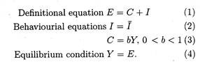
Here b is the MPC and investment is autonomous. Hence it is independent of national income. So it is taken as fixed in equation (2).

Now if we substitute equation (1) into equation (4) we get:

Y = C + I (5)

Further substitution of equations (2) and (3) in equation (5) yields the following:

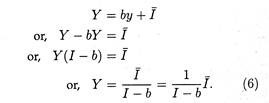
Here b is a constant and I is also a constant. Therefore, both the terms on the right hand side are constant. Thus Y in equation (6) is indeed the equi­librium level of income.

The Saving-Investment Approach:

The same condition will be obtained if we use the second approach, viz., the saving-investment ap­proach.

We may now use the following equation:

 

 

 

Here s is the MPS. All other terms have their usual meaning and significance. Substituting (8) and (7) into (9) we get:

 

 

 

 

 

 

Equation (10) states that the equilibrium level of national income is found out by dividing autonomous expenditure by the MPS.

It is now easy to verify that the two forms in which equilibrium income are stated, (6) and (10), are equivalent. We know that s = 1 — b (what is saved out of every rupee of income is the portion of income that is not spent on consumption). By substituting (1 — b) for s in equations (10), we obtain equation (6).

Alternatively if we substitute s for (1 —b) in equa­tion (6), we arrive at equation (10). This shows that (6) and (10) are equivalent. They are just two alterna­tive ways of stating the same (or equilibrium) level of national income implied by the Keynesian model.

Problem 3:

Suppose the household sector’s planned consumption is C = Rs. 50 + 0.80Y_d and intended investment is Rs. 50. In the absence of a govern­ment sector and taxes, the value of output equals the household sector’s disposable income so that Y_d = Y. Given the specified spending plans, find out the equi­librium value of national income.

Solution:

Equilibrium condition is: Value of output = planned aggregate spending

Y = C + I

Y = (Rs. 50 + 0.80y) + Rs. 50

Y- 0.80Y = Rs. 100

Y(1 – 0.80) = Rs. 100

Y(0.20) = Rs. 100

Y = Rs. 100/0.20

Y = Rs. 500

Problem 4:

Suppose C = Rs. 50 + 0.80Y_d; I = Rs. 50; Y = Y_d. Intended saving equals Y_d — C. Thus, the saving function is S = —Rs. 50 4- 0.20Y.

[S = Y_d — C; Y_d = Y: S = Y-(Rs. 50+0.80y)].

Find out the equilibrium value of national income.

Solution:

According to the leakages-injections approach, the equilibrium condition: Intended saving equals in­tended investment.

Problem 5:

Suppose derived consumption is C + bY: I = Ī. Find equilibrium income when C = Rs. 50: b = 0.80 and Ī= Rs. 90.

Solution:

(b) Substituting, we have Y = (Rs. 50+Rs. 90)/ (1 – 0.80); i.e., Y = Rs. 140/0.20 = Rs. 700. the equilibrium level of income.

Generality of the Results:

From Keynes’ model we have arrived at a general result that national income is in equilibrium where aggregate planned expenditure is equal to actual out­put (i.e., actual national income). Graphically this is shown by the intersection between the aggregate ex­penditure line and the 45° line.

It also follows from the Keynesian model that national income equilibrium occurs where planned saving equals planned investment.

Graphically, this is shown by the intersection of the 5 and I lines. In a two-sector economy where saving is the only de­sired leakage and investment is the only desired injec­tion national income is in equilibrium where leakage equals injection, i.e., where S = I. However, this is not a general result in the sense that it does not always hold. We may now examine why it is so.

Saving-Investment Equality vs. Saving-Investment Equilibrium:

The saving and investment decisions are made by different groups of people. So there is no necessary reason why house­holds should decide to save exactly the same amount as firms decide to invest. However, in the simple

Keynesian model, national income is in equilibrium when planned saving is equal to planned investment. It implies that there is a mechanism that ensures that households end up desiring to save exactly what firms desire to invest. The mechanism is in the change in national income that occurs when desired saving is not equal to desired investment.

The explanation of the apparent conflict is the essence of the Keynesian theory of income determi­nation. The classical economists believed that saving was always equal to investment due to the operation of the Say’s Law of Markets.

But Keynes argued that there was no reason why the amount that house­holds wish to save at any give level of national income should be equal to the amount that firms wish to in­vest at the same level of national income. But when the two are not equal, certain forces in the economy will be at work that cause national income to change in the desired direction. In fact, income change con­tinues until the two become equal.

In Fig. 34.4 we have put a value upon savings and investment and we see that they are equal to each other. The economy is therefore in equilibrium be­cause injections are equal to leakages (withdrawals).

Since the amount withdrawn (S = 300) is equal to the amount injected (I = 300) there is no tendency for the level of income (Y) to change. The economy is said to in equilibrium. It is in this context that we have to distinguish between planned and actual values.

Planned and Actual Values:

It was Keynes who first noted that what people plan to do and what they succeed in doing may be two different things. If, for instance, people suddenly start saving more, their spending on consumption goods would fall. So stocks which are a form of investment go up due to a rise in saving. Thus, actual (ex-post) sav­ings are equal to actual (ex-post) investment.

On the contrary, if people save less and spend more on con­sumption goods, business firms will find their stock levels falling. Thus, a fall in saving will lead to a fall in investment and actual savings would once again be equal to actual investment.

This point may be illustrated in the following manner. Income is made out of expenditure on con­sumer goods and that on capital goods.

So, from the expenditure side, national income may be expressed as:

Y = C + I

where C is the demand for consumption goods and I is the demand for capital goods. However, from the output side, income received by people is divided be­tween consumption and saving.

Thus, we can write:

Y = C + S

where C stands for the supply of consumption goods and S for the supply of capital goods.

Since national income = national expenditure = national output, we can write:

Y = C + I = C + S

or, C + I = C + S

By cancelling out C from both sides we get:

I = S

or actual I = actual S.

This is known as saving-investment equality and is always true because it is a definitional identity rather than an equation. It follows from the national in­come accounting system. However, in most real life situations, planned savings are likely to differ from planned investment.

There are two reasons for this:

(1) Savings and investment are different activities car­ried out by different groups of people and

(2) The motives for savings and investment are diverse.

In fact, for these two reasons, the savings and invest­ment plans of the two groups may remain unfulfilled and there may be divergence between planned sav­ing and planned investment. In Keynes’ model of a two-sector economy changes in factor income cause changes in the plans of Consumers and producers un­til the two sets of plans are reconciled.

Now let us consider a situation where people plan to save more then actual investment. This will cause national income to fall because withdrawals ex­ceed injections.

The fall will continue until people can no longer afford to save more than what is invested by firms. Conversely, if planned (desired) investment is greater that desired saving, national income would rise. This, in its turn, would raise the volume of sav­ing. The process would continue until savings once again coincide with investment.

Thus, the prediction is that for national income equilibrium to exist it is necessary for planned (ex- ante) S to equal planned (ex-ante) I. This is known as saving-investment equilibrium,see Table 34.3 below.

The table gives a consumption function, from which saving plans can be obtained. Assuming that planned investment is autonomous and that all household plans are realised, an equilibrium level of income can be calculated.

When income is 500 the consumption spending is 450 and saving is 50. At this level of income autonomous planned investment is 50, thereby bringing to­tal planned expenditure (consumption + investment) equal to the level of output (or income). With planned saving and investment being equal, the economy is in-equilibrium.

However, at the higher level of income (600), planned saving exceeds planned investment result­ing in planned expenditure falling below planned in­come. As the rate of production exceeds the rate of sales by 20% the level of stock will rise thereby resulting in a rise in unplanned investment. Any stock changes are regarded as changes in investment.

At this stage realised investment, made up of planned and unplanned investment, will still be equal to re­alised saving, but the discrepancy between the inten­tions of savers and investors will result in the level of income falling back until it reaches the equilibrium level of 500.

If income were 400 the consumption schedule would indicate that 370 would be consumed and 30 saved. With planned investment exceeding planned saving, planned expenditure would exceed planned income resulting in a fall in the value of stocks (in­ventories). The fall in stocks can be regarded as un­planned disinvestment, giving a realised investment figure of 50 – 20 = 30 (which is the same as actual saving).

The above argument may also be expressed graphically. Since the saving line in Fig. 34.5 does not everywhere coincide with the investment line, planned saving of the household sector does not al­ways equal planned investment of firms.

However, the two lines intersect at only one point and the point at which the equilibrium level of national income oc­curs. For example, in Fig. 34.5, e is the equilib­rium point of national income.

Since the S line intersects the I line at this point, national income Y_e is in­deed the equilibrium level of income. If investment exceeds saving by cd, when income is Y₁, the ex­pansionary forces behind the national income will be stronger than the contractionary forces and national income will rise.

Oppositely, if saving exceeds invest­ment, when income is income will fall for obvious reasons. Both of these are disequilibrium situations.

Thus, if national income is at either Y₁ or Y₂, it will move away from these levels. Only at Y_e, it is in equilibrium and only at this level of income desired (planned) saving is equal to desired (planned) invest­ment.

In this context the following quote from R. G. Lipsey becomes relevant: “These is no reason why de­sired saving should equal desired investment at any randomly chosen level of income, but when they are not equal in the two-sector economy, national income will change until they are brought into equality.”

So we have identified the forces that determine equilibrium national income.

Problem 6:

Suppose desired consumption equals Rs. 40 + 0.75Y. and desired investment is Rs. 60. (a) Find the equilibrium level of income, the level of consumption and saving at equilibrium, (b) Show that at equilib­rium planned spending equals the value of output and desired saving equals desired investment.

Solution:

 

 

 

 

 

 

 

 

 

 

 

 

(b) Planned spending equals the value of output

C + I = Y

Rs. 340 + Rs. 60 = Rs. 400.

Planned saving equals planned investment

S = I

Rs. 60 = Rs. 60.

Problem 7:

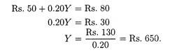
Suppose planned consumption equals Rs. 50 + 0.80Y_d; I= Rs. 80; and Y_d = Y since there is no government sector, (a) Derive an equation for the saving function, (b) Calculate equilibrium value of income by equating desired saving and desired in­vestment.

(a) Planned saving equals Y_d — C; and since C = Rs. 50 + 0.80Y_d,

S = Y_d– (Rs. 50 + 0.80Y_d)

S = -Rs. 50 + 0.20Y_d.

(b) The equilibrium condition is determined by equating planned saving and planned I; thus