Oligopolistic Models of Intra-Industry Trade | Economics

In case of intra-industry trade models, it was assumed that the number of firms in the manufacturing sector in each country was large. There is another group of models in which the number of firms in the manufacturing sector is supposed to be small. Such models are termed as the oligopolistic models. The most significant element in the oligopolistic models is the strategic interdependence of firms in the market.

Each firm in the market recognises that its price and output decisions are likely to effect the profits of other firms. The rival firms are likely to react to those decisions. The reactions of the rivals to the price-output decisions of the given firm are called as ‘conjectural variations’. The alternative models of oligopoly emerged only on account of the nature of conjectural variations, i.e., how the rival firms react to price and output decisions of one another.

We shall discuss below some oligopolistic models of intra-industry trade:

1. The Brander-Krugman Model:

This model related to intra-industry trade has been developed by J.A. Brander and P.R. Krugman.

Assumptions:

This partial equilibrium model rests upon the following main assumptions:

(i) There are two countries, which are identical in all respects.

(ii) The commodity is homogeneous.

(iii) There is one producer in each of the two countries.

(iv) Each producer has equal costs of production.

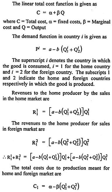
(v) Total cost function is linear in the two countries.

(vi) The domestic demand function is identical in the two countries.

(vii) Both the firms display Cournot behaviour i.e., each firm assumes that the supply of the rival firm will remain constant.

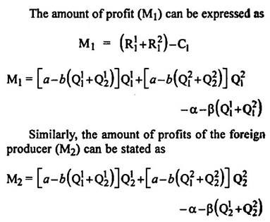
Following the Cournot model, each producer will determine his sales in two markets on the assumption that the sales of the rival will remain unchanged, such that he could maximize his profits.

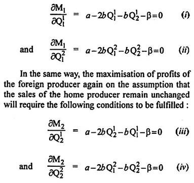
For the maximisation of profits of the home producer, the following conditions must be satisfied:

By solving equations (i) and (iii), equilibrium sales in the home market can be determined. Similarly by solving equations (ii) and (iv), the equilibrium sales in the foreign market can be determined. Each firm will produce, in the state of equilibrium, equal quantities. Each one of them will sell one half of that output in the home market and one half in the foreign market.

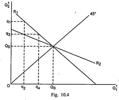
It is possible to show the equilibrium in the home market through Fig. 10.4.

In Fig. 10.4., sale by the home producer in the home market (Q¹₁) is measured along the horizontal scale and sale by the foreign producer in the home market (Q¹₂) is measured along the vertical scale.

A 45° line is drawn from origin. R₁ is the reaction curve of the home producer and R₂ is the reaction curve of the foreign producer. Suppose initially the foreign producer attempts to sell q₁ quantity in the home market. Given the foreign sale q₁ and reaction curve R₁ of the home producer, the profit- maximising sale by the home producer in the home market is q₂.

Given the sale q₂ by the home producer and foreign producer’s reaction curve R₂, the latter will choose to sell the quantity q₃. The reaction of the home producer to this sale by foreign producer, given the reaction curve of R₁, will be to sell q₄ quantity. The equilibrium will take place at the intersection of R₁ and R₂ exactly at the 45° line. In the equilibrium situation, the home producer and foreign producer will sell equal quantities Q₀ in the home market. It is possible to make similar analysis also for the foreign market.

The Brander-Krugman model is different from standard Cournot duopoly model in only one respect that the producers belong to two different countries, so that trade between them is the intra- industry trade.

2. The Reciprocal Dumping Model:

The reciprocal dumping refers to a situation in which dumping leads to two-way trade in the same product. The possibility of reciprocal dumping was first of all considered by James Brander. Suppose there are two monopolists one in the home country and the other in the foreign country. The two producers produce the same product. It is also assumed that these two firms have the same marginal cost. The same cost of transportation is present between the two countries. If they charge the same price, the trade will not take place between them.

However, the possibility of dumping may lead to the emergence of international trade. Each of them may have a higher price in its domestic market and a relatively lower price in the foreign market. It will afford opportunity for both the producers to maximise their profits and dispose of a part of their production in the foreign market.

Maintaining price differentials in the home and domestic markets, the two producers will have two- way trade in the same product. For instance, the automobile firm in country A will sell automobiles in country B and the automobile firm in country B will sell automobiles in country A. Thus, the reciprocal dumping will tend to increase the volume of trade in goods that are not quite identical.

The reciprocal model of trade is associated with the names of Brander and Krugman. They introduced transport costs into the duopoly model and assumed that some proportion of exports (g) is absorbed by these changes where 0 < g < 1. This model is also referred as “iceberg” model of transport costs.

The profit function of each producer has to be modified, if the transport costs are introduced.

The profits for the home producer can now be expressed as:

Similarly, the profits of the foreign producer can be expressed as:

Since the home producer reacts to what his competitor sells in that market and not to what the competitor produces for that market, there will be no change in either producer’s reaction function. Each producer’s reaction function for his export market, however, must get affected.

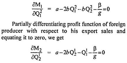
Now partially differentiating home producer’s profit function with respect to his export sales and equating it to zero, we get:

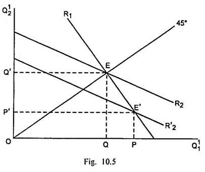
The equilibrium in the home market with transport costs can be explained through Fig. 10.5.

In Fig. 10.5, sales of home producer in the home market (Q¹₁) are measured along the horizontal scale and sales made by foreign producer in home market (Q¹₂) are measured along the vertical scale. A 45° line is drawn from origin.

Originally in the absence of transport costs, the reaction curve of the home producer is R₁ and that of the foreign producer is R₂. The equilibrium is determined by the intersection of R₁ and R₂ curves at E where the sales of the home producer and foreign producer in the home market are equal (Q = Q’).

Since g is less than unity, β/g will be greater than β. It will cause a shift in the foreign producer’s reaction curve down from R₂ to R₂‘. So R₂‘ is the foreign producer’s reaction curve when transport costs are present. The equilibrium in the home market, when transport costs are present, is determined at E’ by the intersection between R₁ and R₂‘ where sales by the home producer in the home market have risen from Q to P but the sales by the foreign producer in the home market have fallen from Q’ to P’.

Fig. 10.5., shows that reduction in the exports of foreign producer to the home country is greater than the increase in sales of the home producer in the home country. Consequently, the price of the product in the home market must increase. This analysis will hold true also for the foreign market.

Given the symmetry assumption involved in the model, there must be the same price in the two markets. Each one of the two producers must be receiving a higher price for sales in the foreign market net of transport costs.