The Specific Factor Model of Trade | International Economics

In this article we will discuss about the specific factor model of trade.

Single Specific Factor Case:

The Heckscher-Ohlin factor endowment theory was put into doubt by the Leontief Paradox. Another objection against the validity of the H-O theory was raised by Stephen Magee. An assumption has been taken in the H-O theory that the factors of production are perfectly mobile within a given country although these are perfectly immobile between the different countries. Magee disputed the contention about mobility of factors in different industries within the same country.

According to him, the difficulty in the inter-industry mobility of factors is created by the specificity of factors. Certain factors are suitable for specific use and these cannot be transferred from one industry to another. Such factors can be called specific factors. Suppose production in a country gets shifted from cotton cloth to steel, no magic wand exists that can convert bales of cotton into iron ore.

The workers skilled in making cloth cannot be absorbed into the steel industry. Even the capital stock employed in cotton textile industry is highly specific in the short period. Over a period, no doubt, it can be diverted from one industry to another. Moreover, the different industries can employ factors in specific quantities.

Suppose two commodities X and Y are produced in a country. Their production involves the use of labour and capital. The supply of labour is fixed for the country as a whole and it is perfectly mobile within these two industries. But each industry employs a specific quantity of capital. Since capital in one industry cannot be substituted for capital in the other country, there can be no way by which price of capital can be equal in two industries. Wages in the two industries can, of course, get equalised. The equilibrium situation from the point of view of labour can be shown through Fig. 9.3.

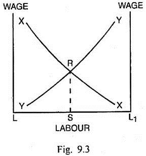
In Fig. 9.3, labour is measured along horizontal scale and wage is measured along vertical scale. LL₁ is the total supply of labour in the country. The supply of labour for X industry is measured to the right of L. For Y industry, it is measured to the left of L₁. Curves XX and YY measure value of marginal products of labour in goods X and Y respectively at different employments of labour. As more labour is employed in industry X, given the fixed stock of capital, the MPL_X falls and XX curve slopes negatively. Similarly curve YY slopes negatively. The curves XX and YY depend upon the technology used, prices of products and specific amounts of capital used in the respective industries.

An increase in input of labour can increase production, if the specific capital is also increased. That can result in shifts in the curve XX or YY. The value of marginal product of labour in X industry is P_X.MPL_X. So long as the cost of hiring an additional worker falls short of P_X.MPL_X, the producer in this industry will employ more and more workers. The expansion of labour input will continue until wage w equals the value of marginal product (w = P_x MPL_x).

Similarly in industry Y, the labour input will be increased until w=P_Y.MPL_y. Ultimately the equilibrium situation occurs at R when LS workers are employed in industry X and L₁S workers are employed in industry Y. In this situation, P_XMPL_X= P_Y.MPL_Y = w = RS. It means wage rate gets equalised in both the industries due to free movement of labour among different industries or sectors within the country.

Changes in Factor Endowments:

Given the prices of two commodities X and Y, a change in the input of mobile factor labour, will result in a fall in price of labour in both the industries and a rise in price of specific factor capital in both the industries. This is quite in contrast with Rybczynski theorem. The effects of changes in factor endowments are analysed through Figs. 9.4 part (i) and (ii).

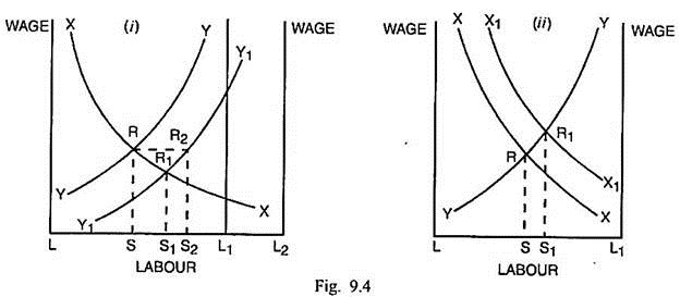
In Fig. 9.4. (i), originally the wage or price of labour is equal at RS (= R₂S₂) in both X and Y industries. As the supply of mobile factor labour is increased by L₁L₂ = RR₂ = SS₂, the curve YY shifts to the right to Y₁Y₁. The supply of labour rises in industries X and Y by SS₁ and S₂S₁ respectively. Since each additional worker has to work with less capital, the MPL in both the industries falls.

Consequently, the price of labour in both the industries declines to R₁S₁ even though the output in both the industries has risen. This is in contrast to Rybczynski theorem. The price of capital in both the industries will increase because each type of capital is being worked with a larger quantity of labour resulting in higher marginal products of capital in the two industries.

Fig. 9.4. (ii) Analyses the effect of an increase in capital specific to industry X. When there is an increase in the quantity of capital in this industry, the labour input remaining the same, the MPL in industry X will increase and the MPL curve shifts from XX to X₁X₁. In order to maintain equality in the values of marginal products in two industries, mobile factor labour must shift from industry Y to industry X by an amount SS₁.

This diversion will raise output in industry X but lower the output in industry Y. The wage rates in both the industries will go up from RS to R₁S₁. The rentals on both types of capital will decline. Such changes are closer to the effects suggested by Rybczynski theorem.

If the two countries are engaged in free trade, given an identical pattern of demand and techniques of production, changes in the mobile factor labour will have no effect upon the pattern of trade. However, as change takes place in the supply of specific factor capital, the outputs of two commodities change in opposite directions. In such a situation, each country in likely to export the good using that country’s relatively abundant specific factor. Such an effect is fully consistent with H-O theorem.

Effect of Price Changes:

The specific factor model analyses also the effect of changes in prices of the commodities upon the returns of the factors. Suppose the price of X commodity rises, it will raise the value of marginal product of X, i.e., P_X.MPL_X in proportion and will cause a shift in the curve XX (See Fig. 9.5) upwards to X₁X₁. There is movement of labour SS₁ from the production of Y to the production of X. The wage rate rises in industry X from RS to R₁S₁. Since the rise in the wage rate is less than that of price of X, the real wage in industry X falls. In the case of industry Y, since the price of Y remains unchanged, the increase in wage rate signifies a rise in the real wage in this industry. Such a conclusion is in contrast with the conclusion given in Stopler-Samuelson theorem.

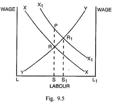
As regards the real return of the specific factor capital, with more labour to work with capital specific to product X, the marginal product of capital will increase. Along with that the return on X-specific capital will increase. In case of commodity Y, less labour is available to work with Y-specific capital. It can result in a fall in return from Y-specific capital.

Two Specific Factors Case:

This variant of specific factor model was developed by Paul Samuelson and Ronald W. Jones. This model involves two commodities, two countries and three factors along with the neo-classical production function. Out of the three factors—land, labour and capital, there are two factors, land and capital, which are specific to the production of, two commodities X and Y respectively. These factors cannot be transferred from one industry to another. Labour is the only factor that is used in both industries.It is mobile between the two industries in each of the two countries.

Assumptions:

This variant of the specific factors model rests upon the following assumptions:

(i) There are two commodities X and Y.

(ii) There are two countries A and B.

(iii) Land, labour and capital are the three factors. The factor land is specific to the production of X commodity. The factor capital is specific to the production of Y. The factor labour is used in the production of both X and Y commodities and it is mobile within the two industries in both the countries.

(iv) There are the conditions of perfect competition in the commodity and factor markets.

(v) There is greater use of labour in country B than in country A.

(vi) Marginal physical product of labour diminishes as the input of labour is increased.

(vii) There are identical production techniques in the two countries.

(viii) Tastes and preferences of the consumers are identical in the two countries.

Since country B makes more use of labour than A, it suggests that B is relatively more labour- abundant than country A. On this basis, the production possibility curve of country A is AA₁ and that of country B is BB₁ as shown in Fig. 9.6. Commodity X (such as wheat) is land-specific and labour-intensive. The commodity Y (such as steel) is capital-specific and less labour-intensive. The slopes of the two production possibility curves show that country A has comparative advantage in the production of Y whereas country B has the comparative advantage in the production of X.

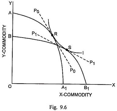
I is the common community indifference curve for both the countries. Before trade, R is the point of production and consumption equilibrium for country A and S is the point of consumption and production equilibrium for country B. The domestic price ratio in country A is represented by the slope of the line P₀P₀ and that of country B is represented by the slope of line P₁P₁.

These lines indicate that commodity X is relatively cheap in country B than in country A and commodity Y is relatively cheap in country A than in country B. As trade commences, the capital-specific country will export its relatively cheap and capital-intensive commodity Y. The land- specific country B, on the other hand, will export its relatively cheap and labour-intensive commodity X. The specific factor model in this way leads to the same conclusion as had been given by the H-O model.

As regards the gain from trade for the specific and mobile factors, Sodersten and Reed point out that the factor specific to the export sector gains and the other immobile factor loses. The mobile factor gains in terms of one commodity and loses in terms of the other commodity so that overall its position may remain almost unchanged.