Models of Intra-Industry Trade | International Trade | Economics

List of models of intra-industry trade: 1. Neo-Heckscher-Ohlin Model 2. Neo Chamberlinian Models 3. Neo Hotelling Models.

1. Neo-Heckscher-Ohlin Model:

The original H-O theory of international trade is not capable of explaining the intra-industry trade. Some writers have still made attempts to explain the intra-industry trade based on factor endowments by establishing link between the product specifications and the different combinations of the basic factors like labour and capital. A prominent attempt was made in this regard by R.E. Falvey in 1981. This model is referred as the Neo-Heckscher- Ohlin model of trade.

Assumptions:

This model rests upon the following main assumptions:

(i) There are two countries A and B.

(ii) There are two industries X and Y.

(iii) There are two factors of production, labour and capital, which are homogenous.

(iv) Labour is mobile between the two industries.

(v) The factor capital is industry-specific.

(vi) The industry X produces an identical product.

(vii) The product of the other industry Y is differentiated.

In this model, it has been recognised that the differentiation in the product Y is based upon quality. Such product differentiation is generally referred as vertical differentiation. The income of the consumer and price of the product determine demand for different varieties of product Y. For the sake of simplicity, it may be assumed that there are two varieties, Y₁ and Y₂, of the product.

Out of them, Y₂ is supposed to be the superior variety. In each time period, every consumer purchases one or both products. At higher levels of income, consumers would buy more quantity of the superior and lesser of the inferior product. At low levels of income, consumers are constrained to spend much of their income on the purchase of inferior product Y₁, even though they have preference for the superior product Y₂.

For producing a superior variety of product Y, a firm must make use of more capital per unit of labour. Let us suppose, the production of one unit of any variety of product Y requires the use of one unit of labour. The input of capital required to produce one unit of any variety of product Y is µ. Higher the magnitude of µ, better can be regarded the quality of the product. In other words, n represents the index of quality.

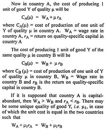
If the unit cost of producing the product of quality n is lower in country A than in country B, i.e., C_A(µ) < C_B(µ), the country A will have a comparative advantage over B in the production of this variety of product. If µ₁ < µ, the comparative advantage of A over B, will hold [C_B(µ) > C_A(µ)], because W_B < W_A.

Thus country A, which is capital-abundant and in which capital is relatively cheap, will have a comparative advantage in producing those varieties of the product Y in case of which quality is superior to the marginal quality. This country will, therefore, export superior varieties of the capital-intensive product. The labour-abundant country B will export both the labour-intensive good and the lower quality varieties of the capital-intensive good.

Instances of such trade can be found in some parts of the clothing industry, where capital-abundant countries tend to export superior quality products to the labour-abundant countries, while importing lower quality products from them. Thus H-O theory can explain the intra-industry trade between the different countries.

2. Neo Chamberlinian Models:

The Neo-Chamberlinian models related to intra- industry trade include the models developed by the writers like RR. Krugman, A. J. Venables, C. Lawrence and RT. Spiller. These models recognise that there is horizontal differentiation of goods. The horizontal differentiation of goods is supposed to occur when the product varieties differ in their characteristics, which may either be actual or perceived.

For instance, the differentiation based upon colour (colour of a cold drink) is actual and the differentiation based upon taste (taste of cold drink) is perceived. It is possible that the individual consumers may have unique ranking of different varieties in accordance with the characteristics of varieties matching their preferences. In this regard, it should be remembered that there can be no such ranking about which there is agreement among all the consumers.

In the present discussion, we shall mainly consider the model suggested by P.R. Krugman.

Assumptions:

In this model, the following assumptions have been taken:

(i) There is only one factor of production, labour, in the economic system.

(ii) Labour is in fixed supply.

(iii) There is a large number of firms but the number is determinate.

(iv) Each firm turns out a different variety of the same commodity, say X.

(v) There is free entry or exit of firms in the market.

(vi) There is no limit upon the number of varieties that can be produced by a firm.

(vii) The average labour requirements decrease with an increase in output.

(viii) Each consumer has the same utility function, in which all varieties enter symmetrically.

The total labour requirements of firm i is measured as:

l_i, = α + β_xi;

Where x_i = Output of variety i of X commodity

β = Co-efficient relating labour requirement and output, and

α = Labour requirement independent of output.

The assumption taken by Krugman that all varieties enter the utility function symmetrically has two implications. First, the consumption of an additional unit of any variety causes the same addition to total utility. Second, there is increase in total utility due to the consumption of more varieties.

The actual utility function suggested by Krugman can be expressed as:

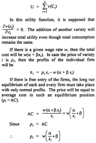
Since the model assumes symmetry, it implies that the price, average cost and output in case of each firm will be the same. In other words, for all the firms, l_i, = l, p_i, = p and x_i, = x.

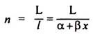
It is possible to determine the number of firms on the basis of the condition that the labour used in the production of all varieties cannot be more than the fixed supply of labour. If each firm employs I amount of labour when l = α + βx and the total fixed labour supply is L, then the number of firms (n) will be-

Since each consumer is assumed to consume exactly the same amount (c) of each variety of the product, the total utility function of the consumer will be expressed as:

U = n v (c)

The total spending on all varieties of the good evidently must be equal to the total payment made to labour.

It is now supposed that there is another country which is identical to the first country is every respect. In the conditions of free trade, absence of transport costs and other barriers to trade, trade will take place between these two countries in the given differentiated product.

A firm in one country that was producing earlier a variety identical to one produced in the other country, will switch over to variety of product that is not being produced by any other firm. This will be done because production cost is identical for it in case of all the varieties and it can dispose of the same quantity of the new variety as it had been doing in the case of the earlier variety.

Since each firm will produce only one variety, it implies that each variety will be turned out in only one of the two countries. Since each country will produce n varieties when the cost of production and sale price is the same as before, the free trade equilibrium will be identical with the equilibrium in the absence of trade.

Since each consumer in each county will now consume an amount 0.5 C of each of n varieties, the total utility for him will be:

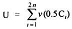
It will evidently signify an increase in the utility of an individual consumer. Although there is same volume of total consumption, yet all the consumers will gain from trade due to the use of a wider variety of goods, there being no loss on production side and real wage remaining exactly equal in the two countries. Thus, the intra-industry trade assumes welfare gain for both the countries.

The intra-industry trade model given by Krugman is indeterminate in one sense. This model, no doubt, leads to the inference that one half of the range of product varieties will be produced by each country, yet it is unable to tell which varieties will be produced by each country.

On the basis of the analysis made in Krugman model, A.K. Dixit and V. Norman observed that the welfare-augmenting intra-industry trade can exist even in the identical economies having horizontal product differentiation and falling average cost of production.

In the category of Neo-Chamberlinian models, we briefly consider another model discussed by A.J. Venables. In this model, there is an extension of Krugman-type model in which there is production of identical product under the conditions of constant costs. This model discusses the possibility of multiple equilibria including also a situation in which one country specialises in the production of homogeneous good, while the other country specialises in the production of differentiated good.

Another model in this context is one suggested by C. Lawrence and P.T. Spiller. It extends the basic model to include two factors of production that are employed to turn out a labour-intensive identical product and a capital-intensive horizontally differentiated product. In this model, it is assumed that the initial factor proportions in the two countries are different and that the firms entering the sector producing differentiated products have to incur substantial initial capital outlay.

Lawrence and Spiller, in this model, gave two major conclusions. First, the number of varieties will increase in the capital- abundant country and their number will shrink in the labour-abundant country. Second, the labour- abundant countries will enlarge the scale of production of identical goods, while the capital- abundant countries will expand the scale of production of differentiated products. These conclusions have much similarity with the conclusions given by the basic H-O model and the model given by R.E. Falvey.

The Neo-Chamberlinian models, mentioned above are restricted on account of their unrealistic and faulty assumptions.

The main weaknesses in these models are as under:

(i) The form of utility function taken in Krugman model discounts the possibility that consumers follow same scale of preferences related to the product varieties.

(ii) It is clearly unrealistic to suppose that the product varieties are completely independent of demand.

(iii) When the firms switch from one variety to another, some adjustment costs have to be incurred but these models ignore such costs.

(iv) Apart from the adjustments costs, the change in product variety may involve some other costs, which again have not been recognised in these models.

(v) These models assume that the opening of trade will not result in the disappearance of any variety. In fact, as new varieties are introduced, some older varieties will disappear altogether from the markets of the two countries.

3. Neo Hotelling Models:

The structure of models referred as Neo- Hotelling models rests upon the approach suggested by K.J. Lancaster. He discussed the characteristic- based model of product differentiation on the basis of which the existence of intra-industry trade could be explained.

Assumptions:

Lancaster’s model is based upon the following main assumptions:

(i) There are two countries that are identical in all respects.

(ii) There are two sectors in the economies of two countries—manufacturing and agriculture.

(iii) The manufacturing sector produces the differentiated good.

(iv) The agricultural sector produces a homogeneous good.

(v) The production is governed by constant returns to scale.

(vi) Out of two factors of production involved, labour is the mobile factor.

(vii) The second factor of production employed in each sector is specific.

(viii) Each consumer has a most preferred or ideal variety for which he has the maximum willingness to pay.

(ix) The demand for a given variety depends upon the price of that variety, income of the consumer and the existence of other varieties.

(x) On the supply side, there is free entry and exit of firms, with firms deciding to produce any variety.

(xi) The cost of producing any variety is the same.

According to Lancaster, the freedom of entry and exit along with equal density of preferences and identity of cost function will lead to the long run equilibrium in which the actual varieties produced will be spaced in an even way along the whole spectrum of varieties. Each variety will be produced in equal quantity and will be sold at the same price such that each firm will be obtaining only normal profits. Lancaster terms this situation as ‘prefect monopolistic competition’.

In the absence of trade, the two countries will produce same varieties in the same quantities. There will also be the same agricultural production, prices and incomes. In other words, there will be the same equilibrium position in both the countries.

If the free trade opens, it amounts to the creation of one country, which is twice the size of either of the two original countries because they are identical. The only difference is that there is a lack of movement of factors of production between them. Each variety, in the case of differentiated product, will be produced by only one firm of only one of the countries and varieties are spaced evenly along the spectrum. The production of each variety will be in the same volume and each will be sold at the same price.

The consumption of all varieties will, however, take place in both the countries. Since the model has been assumed to involve symmetry, exactly half of the varieties will be produced in each country. Half of the production by each firm will be sold in the home market and the remaining half will be exported to the other country. In other words, half of the consumers in each country will have preference for the domestic variety and half of them for the variety produced in the other country.

There will be no trade in agricultural goods. Trade must, however, be balanced as each country exports same number of goods in the same volume and the same price. In this connection, it may be pointed out that, like Krugman model, no prediction can be made about which varieties will be produced by each country.

When trade commences, the expansion in output would lower average cost resulting in super-normal profits. There would be entry of new firms, each one of them producing a new variety. Thus, the new equilibrium will be established with a large number of varieties than before. Even in this situation, the varieties are spaced evenly along the spectrum.

The trade equilibrium for a typical firm in the manufacturing sector before and after trade can be shown through Fig. 10.2.

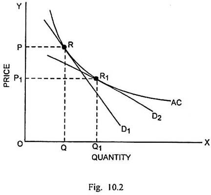
In Fig. 10.2., quantity is measured along the horizontal scale and price along the vertical scale. AC is the average cost curve. In the absence of trade, D₁ is the demand curve. Long run equilibrium of the firm is determined at R where quantity produced is OQ and price is OP. As the trade commences, the increased number of varieties will tend the demand curve to shift down.

Since the adjacent varieties become more close in the spectrum of varieties, that will make the demand curve more elastic. So the new demand curve is D₂. The long run equilibrium after trade will take place at R₁ where the output OQ₁ will be higher and price OP₁ will be lower because price remains equal to average cost.

The welfare effect of trade has been analysed by Lancaster in the case of consumers and producers. There will be some consumers, who can be turned as borderline consumers. They will be on the margin between purchasing one or the other of the two adjacent varieties. The demand curve in the case of such consumers is the conventional negatively sloping demand curve for the variety consumed by them. In their case, the consumer’s surplus gain will result from consuming the given variety.

Since consumers are evenly distributed along the spectrum, there must be the same level of consumer’s surplus for all the borderline consumers. A consumer, in case of whom the ideal variety is closer to the variety being produced, will consume more of the variety than a borderline consumer, will derive larger consumer surplus. The largest consumer surplus will be enjoyed by those consumers in case of whom the ideal variety coincides with the variety being actually produced.

When the trade takes place and the number of varieties available increases by exactly 50 percent, the borderline consumers will become better off for the two reasons. Firstly, they can now purchase a variety, which is closer to their ideal variety. Secondly, since price of each variety is lower than before, they will increase consumption and derive greater consumer’s surplus.

There are, at the same time, some consumers who are no longer able to buy their ideal variety. In their case, it is difficult to generalise whether they will gain or lose in satisfaction. It is possible that some consumers become worse off after trade. Although distributional change due to free international trade will be quite complex, yet the aggregate consumer’s surplus is likely to be greater than before trade owing to the availability of a larger number of varieties at the lower price.

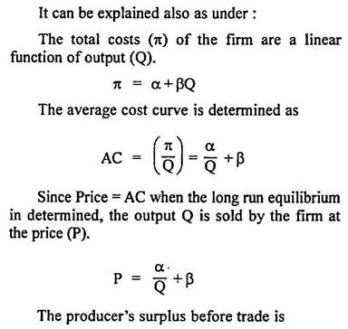
As regards the effect on producers, assuming that there is a linear total cost function and that the number of varieties increases by 50 percent, the analysis can be made with the help of Fig. 10.3.

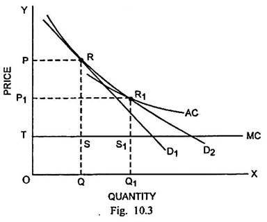
In Fig. 10.3, given the linear total cost function, the average cost curve (AC) slopes negatively. The marginal cost curve (MC) is horizontal. D₁ is the demand curve for the autarchy variety. It is tangent to AC at R. The firm will produce the quantity OQ and sell at OP price. The producer’s surplus is given by the area PRST.

After trade, the demand curve is D₂. The tangency between D₂ and AC curves takes place at R₁ where quantity produced is OQ₁ and price is OP₁. The producer’s surplus after trade is P₁R₁S₁T. Since P₁R₁S₁T is equal to PRST, there is neither net gain nor less to the firms and the producer’s surplus remains unchanged.

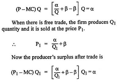
Thus, the producer’s surplus remains unchanged even after trade. In case, the cost function is not linear, there can be the possibility of rise or fall in producer’s surplus.