Short Run Supply Curve of a Competitive Firm and Industry (With Diagram)

Let us learn about the short run supply curve of a competitive firm and industry.

Supply is the quantity which is offered for sale at a given price at a particular time. The supply curve shows the maximum quantities per unit of time which sellers will place in the market at various prices. At a higher price, a greater quantity will be supplied and, at a lower price, a smaller quantity will be supplied.

Recall that the supply of a commodity is a derived function. It is derived from the cost function. It is said that all the supply curves are cost curves, but all cost curves (AFC, AVC, AC and MC) are not the supply curves. Under perfect competition, in the short period, only MC curve is the supply curve.

As is known to all, the MC curve is U-shaped having both negative and positive slopes while supply curve is positive sloping. So we must not consider negative or downward sloping portion of the MC curve. Only rising portion (i.e., upward sloping) of MC is the supply curve. To be more specific, rising portion of the MC the that lies above the AVC curve is the supply curve of a competitive firm in the short run.

Under perfect competition, a firm will produce that amount of output when P = MC. As price is given to a firm, the price line becomes parallel to the horizontal axis.

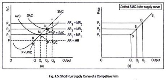
This amounts to saying that the demand curve or the AR curve that coincides with the MR curve becomes perfectly elastic. In Fig. 4.5 (a) AVC, SAC and SMC are the average variable cost curves, short run average cost curve and short run marginal cost curve, respectively.

At a price OP, the firm is in equilibrium at point R since at this point all the conditions for equilibrium are satisfied. Corresponding to this equilibrium point, the firm produces OQ output. The total revenue that the firm expects to earn from the sale of OQ output is OPRQ. But costs are higher than revenue since AVC and SAC curves lie above the OP price line.

At this output, the firm not only fails to cover up its fixed cost but also a part of the variable cost. As AVC exceeds price, the firm should go out of business. So, when price is below AVC (i.e., P < AVC), the short run equilibrium output is zero.

At a price OP₁, the firm reaches equilibrium at point M where P = MC. It produces OQ₁ output and earns revenue to the extent of OP₁MQ₁.

At this output level, though cost exceeds revenue, the firm manages just its variable costs only. It does not cover up its fixed costs. Even then the firm will continue production in the short run in view of producing larger output in the future. The firm expects to manage fixed costs in the future.

At the price OP₁, however, MC = minimum AVC. The point at which MC = minimum AVC is known as the ‘shut-down point’ or the ‘closing-down point’. Note that the firm at the shut-down point is indifferent between operating and shutting down.

The firm has to apply its judgement whether it will stop production at this point in the short run or continue production with the hope of recovering some costs (fixed) in the short run. In view of this, shutdown point is also referred to as ‘zero contribution margin’. Below the shut-down point, the firm experiences negative contribution margin.

At a price OP₂, the firm covers up not only variable costs but also fixed costs since, at point N, it is seen that MC = minimum SAC.

Corresponding to the price OP₂, the equilibrium quantity of output is OQ₂, total revenue is OP₂NQ₂, total cost is OP₂NQ₂. As costs equal revenue, the firm must go on producing. At point N, MC = minimum SAC. This point is called ‘break-even point’. Similarly, at price OP₃, the firm will produce and supply OQ₃ since it earns excess profit.

Points S, B and D of panel (b) are the points at the prices OP₁, OP₂ and OP₃, respectively. By joining these points, we get a curve known as the supply curve, SS₁.

This curve corresponds to SMC curve above the AVC curve of panel (a). Thus under perfect competition in the short run, MC curve that lies above the AVC curve is the supply curve. Or MC curve above the shut-down point is the supply curve. Supply drops to zero if price of the commodity falls below AVC.

However, there are numerous firms in a competitive industry, each producing that quantity of goods where its MC curve intersects the horizontal AR = MR curve. Now, all firms sell the product at the same price.

Therefore, it is apparent that the industry supply curve—of course, in the short run under perfect competition—is equal to the horizontal summation of all firms’ supply curves or MC curves above the minimum point of the AVC curve.

Thus, like the individual supply curve, short run industry supply curve is upward sloping. It is drawn in the same way as we draw the market demand curve from the demand curve of an individual.

In the words of R. G. Lipsey:

“The supply curve for a competitive industry is the horizontal sum of the marginal cost curves of all the individual firms in the industry.”