Notes on Aggregate Supply and its Component!
Aggregate supply is the money value of total output available in the economy for purchase during a given period. When expressed.
In physical terms, aggregate supply refers to the total production of goods and services in an economy. It is assumed that in short run, prices of goods do not change and elasticity of supply is infinite.
At the given price level, output can be increased till all resources are fully employed.
ADVERTISEMENTS:
If we go deep, we will find that aggregate supply is represented by national income. How? We know that the money value of final output is distributed as rent, wages, interest and profit among factors of production which help to produce the output. From producers’ point of view, it is the cost of producing goods and services which they must recover from sale of output; otherwise, they will not produce the output.
Since the sum of factor incomes (rent, wages, interest and profit) at national level is called national income, therefore, aggregate supply (AS), output and national income are same. Alternatively, AS = Y where Y is national income. Thus, income or total output measures the aggregate supply of goods and services.
Aggregate Supply = Output = Income
ADVERTISEMENTS:
Components:
Main components of aggregate supply are two, namely, consumption and saving. A major portion of income is spent on consumption of goods and services and the balance is saved. Thus, national income (Y) or aggregate supply (AS) is sum of consumption expenditure (C) and savings (S).
Put in the form of an equation:
ADVERTISEMENTS:
AS = C + S, i.e., Y = C + S
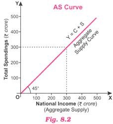
AS curve is depicted in the Fig. 8.2 Aggregate supply or national income is shown on X-axis and total spending (Consumption + saving) on Y-axis. AS curve is artificially represented by a 45° line from the origin why? Because every point on this line is equidistant from X-axis and Y-axis taking same scale on both the axes, i.e., each point on this line indicates Expenditure (AD) = Income (AS).
Thus 45° line (also called a Guide line) helps us to identify equilibrium when two variables are to be shown graphically equal. That is why AS curve is represented by a 45° line so that when AD curve intersects it, AD becomes equal to AS. Thus, every point on 45° line represents AD = AS (i.e., equilibrium).
Again, 45° line implies that the sum of consumption and saving (C -I- S) is always equal to the level of income (Y). Another point to be kept in mind is that since technology is assumed to be constant during short period, output (or aggregate supply) can be increased only by employing more resources, mainly labour. Thus, aggregate supply increases in direct proportion to increase in employment.
Here, Classical and Keynesian concepts of aggregate supply need special mention.
Classical and Keynesian Concepts of Aggregate Supply:
Classical Concept of Aggregate Supply:
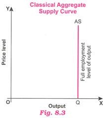
According to Classical, aggregate supply is perfectly inelastic with respect to price level which means changes in price level have no effect on aggregate supply. It is due to J.B. Say’s law of market and wage price flexibility. As a result, Classical aggregate supply a curve is a vertical line parallel to Y-axis at full .s employment level of output as shown in the adjoining Fig. 8.3.
The curve AS is aggregate supply curve and OQ is the full employment level of output. Clearly, vertical shape of aggregate supply curve indicates that changes in price level have no effect on aggregate supply because full employment level of output remains the same at OQ.
Keynesian Concept of Aggregate Supply:
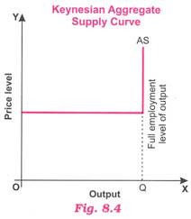
In Keynesian approach, aggregate supply is perfectly elastic with respect to price level till full employment level of output. It means firms are willing to produce any amount of output at the prevailing price level till full employment level of output is reached.
Beyond this point, further increase in production is not possible because all resources in the economy are already fully employed (used). As a result, aggregate supply curve AS, then, becomes perfectly inelastic at full employment level of output as shown in the adjoining Fig. 8.4. Aggregate demand determines the levels of output, income and employment as level of aggregate supply is constant and given in short-run.


