Term Paper on Portfolio Theory | Investment | Financial Economics

Here is a term paper on ‘Portfolio Theory’. Find paragraphs, long and short term papers on ‘Portfolio Theory’ especially written for school and college students.

Term Paper # 1. Introduction to Portfolio Theory:

Two basic principles of finance form the basis of portfolio theory, namely, time value of money and the safety of money.

Rupee today is worth more than rupee of tomorrow or a year hence and as parting with money involves the loss of present consumption it has to be rewarded by a return commensurate with time of waiting. Secondly, a safe rupee is preferred to an unsafe rupee at any point of time. Due to risk aversion of investors, they feel risk is inconvenient and has to be rewarded by a return. The larger the risk taken, the higher should be the return.

Present values and future values are related by a discount factor comprising of firstly the interest rate component and secondly the time factor. The future flows are to be discounted to the present by a required rate of discount to make them comparable and equal in value. As regards the risk factor, there is a direct relationship between the expected return and unavoidable risk. Avoidable risk can be reduced or even eliminated by measures like diversification.

Investment and disinvestment activities should be examined. The basis for these activities is the income and consumption of these economic units. If Y is income and E is expenditure then savings is (Y – E) and borrowing is (E – Y) lending of savings arises if (Y – E) is positive.

Investment activity is based on three components, namely, the following sources of investment:

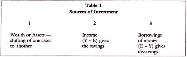
Investment choice depends on firstly the available alternatives, opportunity set, and secondly, the preferences of investors reflected in their indifference curves. The objective of all investors is to achieve the maximum level of utility or consump­tion during any period. The constraints are set by the above three sources. The available opportunities are set by the alternatives open to him, given his preference. Some of them are riskless and with certainty and others are risky and uncertain.

Let us take the case of choices with certainty first. The investor has an income of Rs. 10,000 per annum in each of the two years. As the savings account in bank pays 4.5%, assume that he can also borrow at the same price, as he can lend. Then what are the alternatives open to him?

In a two period simplified model he has three alternative choices open to him. (a) consume in both periods Rs. 10,000 of income, (b) consume less in the first period to save and lend, and (c) consume more in the first period by borrowing and reduce consumption in the subsequent period.

Term Paper # 2. Conditions for Portfolio Theory:

i. Conditions of Certainty:

The equilibrium point is at the point of intersection between the indifference curves (investor preference) and the opportunity set, as shown below:

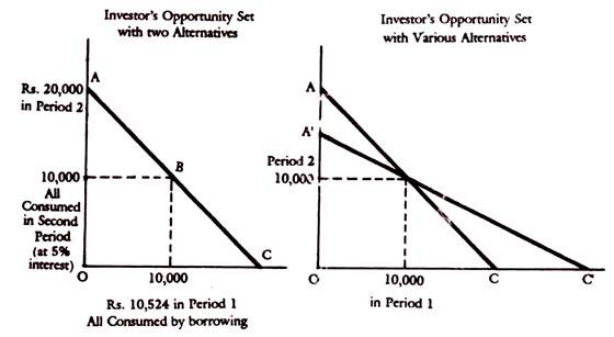
Graphically the opportunity set and investor preferences or utility curves under certainty can be shown as follows:

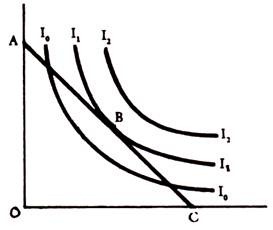
The equilibrium point is set at B on the Indifference curve I_I, the point which is maximum possible for the given oppor­tunity set, given by the line A.C.

ii. Opportunity Set with Uncertainty:

With uncertainty, there can be vari­ous probabilities for the outcome. Then there should be an estimated outcome or the average return and also a measure of the variance of observations over the ave­rage. There can be say many probabilities for the risks expected for the same mean return. The variance of the return from the mean or risk may be different, as seen from the Table 2.

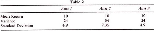
Average return is the mean, which is generally used to measure the expected value. If we know the returns probable for each of the outcomes or events and their probabilities, we can calculate the average, by giving the weights to the returns by the probabilities assigned to them.

Take the following example:

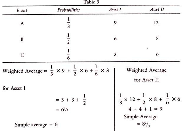
Let the portfolio be of three securities and the market conditions are good, indifferent and bad. Under each of the market conditions expected returns, their mean and deviations can be calculated to derive their covariance.

The table below gives an illustration:

Similar tables can set out for deviations between Asset (1) and (3) and (1) and (4) and soon. The above table gives only for Assets (1) and (2).

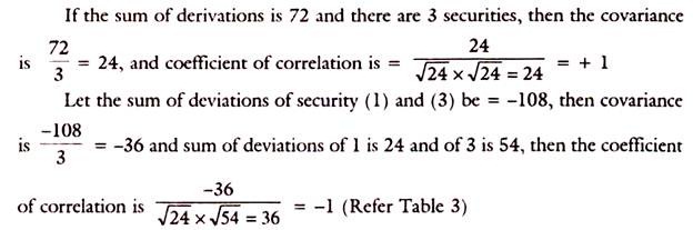
Thus, the coefficient of variation changes between + 1 and -1 and a matrix of covariances between 1 and other assets and between 2 and other assets etc., can be worked out and presented.

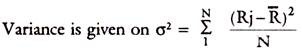
The formula for variance is as follows:

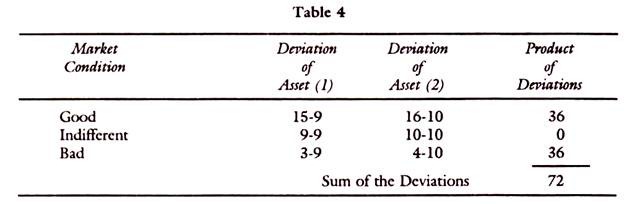
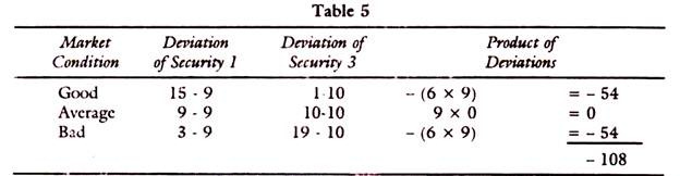
For illustration take the following table for deviations between assets (1) and (3):

Total of squared deviations for security (1) is = 36 + 0 + 36 = 72

Variance = 72/3 = 24

Total of squared deviations for security (3)

81 + 0 + 81 = 162

Variance = 162/3 = 54

Let us study covariance now.

The sum of deviations between assets 1 and 3 in -108.

Then,

Covariance is -108/3 = -36

Correlation coefficient between (1) and (3)

is = -36/√24 * √54 = 36 = -36/36 -1

Risk Measure of Dispersion:

The variability of returns can be from zero to infinity, which is most risky and on the other hand, a safe and fixed income is least risky. This variability or dispersion is measured by the deviation of the actual or expected from the mean or average.

If average is R and observations are R₁, R₂, R₃ … R_n, then-

Standard deviation is the square root of it, namely √σ² = σ

Another factor which influences the portfolio risk is the covariance of returns R₁ to Rn, where R. is the expected return on asset 1 and so on. Covariance is a measure of how returns on two or more assets move together or their inter­relations. If it is positive, they move in the same direction and if it is negative they move in opposite directions. If the positive and negative deviations are unrelated or offset covariance is zero.

Symbolically, Let Pi be correlation coefficient, then-

Pi = σ_ij/σ_iσ_j ; where i and J are the assets and o is the standard deviation.

The numerator a_ij is the covariance and cri is the standard deviation of i and a, is the standard deviation of J asset. Thus, Pi value can vary from + 1 to – 1.

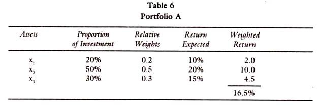
The return on a portfolio is the weighted average of the return on individual assets.

Suppose if the investor has three assets x₁ x₂ x₃ in his portfolio, in which the returns and the proportion of his investment is given as in the following table:

In a similar manner the investor has to assess the expected returns on different portfolios and in different combination of assets to arrive at the proper choice of the portfolio suitable to him. All these combinations will give him the opportunity set. He chooses one set among them with the least risk.

Risk, is measured by variance or standard deviation for an individual security and for the portfolio the covariances among securities are taken into account.

In terms of symbols,

Let σ_i² be the variance of Asset 1

σ₂² be the variance of Asset 2 and so on

x₁ is the proportion invested in Asset 1 ,

x₂ is the proportion invested in Asset 2 and so on.

σ₁₂ is the covariance of Assets 1 and 2

σ₁₃ is the covariance of Assets 1 and 3 and so on.

In our example, let us take two Assets only then the formula for variance (Risk) of portfolio is-

σ_p² = x₁² σ₁² + x₂² σ ₂². + 2 x₁ x₂ σ₁₂

If we plug in some figures, given in the above illustrations, and the proportion invested are assumed is 60% and 40% in Asset 1 and 2 respec­tively, then,

x₁ = 0.6. σ₁² = = 24 and σ₁₂ = – 36

x₂ = 0.4 σ₂² = 54.

Then the risk or variance of portfolio is given as σ_p² –

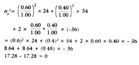
By the above combination of asset (1) and asset (2) we arrived at a zero Risk portfolio, which happened due to the compensating positive and negative covariances, which exactly coincided in values. Otherwise, by such exercise we can arrive at combinations of various degrees of risk and choose the least risk combination. The combinations with the same degree of risk will give the investor’s utility or indiffer­ence curve. Risk also varies with the number of scrips in a portfolio due to possible diseconomies of scale.

Term Paper # 3. Number of Securities in a Portfolio:

There is no rigid rule on the optimum number of scrips or assets in a portfolio. That depends on the amount of fund, investor’s or fund’s goals, risk tolerance and their preferences, and a host of other factors. The unsystematic risks relating to the company can be reduced as shown above, by inclusion of securities, whose covariances among themselves would offset each other, so as to reduce the risk even to zero. That is an extreme case, but normally proper diversification can reduce the risks to the minimum of any portfolio.

Normally for individuals, the risk return management is optimum for 10 – 15 companies, as studies on the Portfolio Management have revealed. In the case of medium size funds of investment companies, portfolio managers, Mutual Funds etc., B.S.E. 30 N.S.E. 50 or even National Index 100 should be enough for a proper management of the fund. The economies of Management of fund reach the optimum for such a number as 10 for individuals and 100 for bigger size funds of investment companies.