Revealed Preference Theory | Commodities | Utility Function | Economics

The theory of revealed preference allows us to use information about consumer choices to inter how the consumer must rank bundles if he is maximizing utility with budget constraints. Alternatively, the revealed preference model explains that how the consumer spends his income with given prices of different commodities. The change in price allows consumer to buy of more or less commodities. But increase in income also helps to buy of more one commodity or buy more of other commodity. Such model is based on certain assumptions.

Assumptions:

Revealed preference theory is based on following assumptions:

1. Consumer spends his entire income on two commodities only.

2. The consumer chooses one commodity for each price vector p and income situation.

3. There is one and only one price p and income combination at which bundle x is chosen by consumer.

4. The consumer choices are consistent. The X⁰ with price p⁰ and if different bundle x¹ is chosen then x⁰ will be no longer feasible alternative.

Model:

Let us assume that P⁰ will be the price vector at which x⁰ can be purchased. The consumer chooses x¹ when X⁰ was chosen. The cost for consumer of consumption bundle is p⁰x¹ > p⁰x⁰. The consumer chooses x⁰ when p⁰x⁰ = M₀. Now the price changes then it increases from p⁰ to p¹. In the economy, such rise in prices is always observed of commodities. At new price level, p¹x⁰ consumer is not happy because he/has to pay more in terms of money.

But his choices are changing and he prefer P¹x⁰ > p¹x¹ then consumer is still better off. Similarly P¹x⁰ ≥ p⁰x¹ implies p¹x¹< p¹x⁰. At new adjustment, the previous bundle of consumption gives more satisfaction to consumer. It also means that P⁰x⁰ ≥ p⁰x¹ → P¹x¹≤ P¹x⁰.

The Weak Axiom of Revealed Preference (WARP):

In the Weak Axiom of Revealed Preference (WARP), we have assumed two commodities. Now x⁰ is chosen at p⁰, M⁰ where B₀ is at equilibrium. Now, X¹ is chosen at p¹m¹. The price effect shows a choice structure, it satisfies the weak axiom of revealed preference. There may be a rational preference relation consistent with these choices.

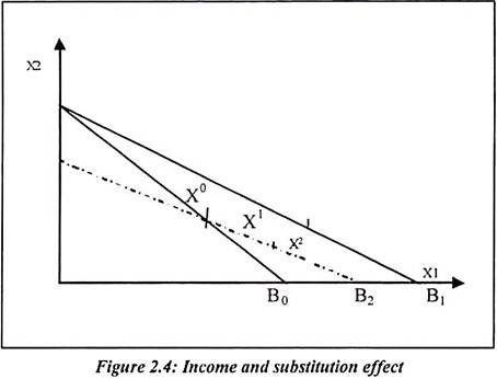
In figure 2.4:

B₀ = It is a consumers’ budget line defined by P₀ and M₀

X₀ = The initial bundle chosen by consumer on B₀

B₁ = It is a budget line after the fall in p₁ with

X¹ = The new bundle chosen on B₁

In the figure, the line B₁ shifts to B₂. The bundle x² is just right to x⁰. Therefore x⁰ and x² is the substitution effect. Both goods are alternatively purchased. The x⁰ and x¹ is income effect which is shown in diagram. It is because of fall in price p₁. The P⁰x⁰ is the price vector and consumption vector. The P¹x¹ is the new price vector and consumption vector. The consumer’s income is adjusted until at m₂x⁰. It can be purchased at the new prices p¹, so that p¹x⁰ = M₂. The price vector p1 and the compensated money income is M₂. The consumer chooses x², it is because all income is spent. We have

The compensating change in M ensures that:

Now x² is chosen because x⁰ is still available to consumers. In routine life, consumer expects to buy new commodities when old commodities exist. It means likeness and preferences changes.

From the equation (10), we have

Here, X² is not purchased by consumer but x⁰ is purchased. It may be because new choice of commodity is not suitable to him.

Now we consider equation (11)

Now, equation (12) can be written as

Subtracting equation (14) from (13) gives the following equation,

And multiplying above equation by (-1) we will have following equation,

This prediction applies irrespective of the number and direction of price changes. In case of a change in the j^th price, only p¹ and p⁰ differ in p_j.

Therefore equation (15) can be written as:

We can also derive Slutsky equation from the behavioral assumption. Therefore M₂ = p¹x⁰ and M₀ = p⁰x⁰ the compensating reduction in M is

The case of Δ in P_i only we have:

Above equation explains that the change in price is equivalent to the change in money income. Government offset the effect of price rise with dearness allowance to public sector workers. Such dearness allowance increases the money income up to the new rise in price level.

The price effect of p_i on X_j is and this can be partitioned into substitution effect (x²_j -x_j) and income effect (x¹_j -x_j). We divide price substitution and income effect by D Pi.

It is as follows:

But from equation (18) we have ΔM = ⎯ Δp_ix⁰_j

.^.. Δp_i = ⎯ ΔM/X⁰_i substituting this into second term of equation (19), we have on the right hand side

Above equation helps us to show the utility maximizing theory of the consumer. The revealed preference theory and utility maximization are equal in their nature.