Problem of Profit Maximization | Firm

To discuss the problem of profit maximisation we shall consider here a simple production process where the firm uses two variable inputs X and Y to produce a single output Q and where the firm buys the inputs at fixed prices r_x and r_Y and sells the output also at a fixed price p. The production function of the firm is

Q = f(x,y)                                  [(8.21)]

And its cost equation and revenue function are

C = r_Xx + r_Yy                             [(8.54)]

R = p x q

The profit (π) of the firm is the difference between its total revenue (R) and total cost (C). Therefore, its profit function is

π = p x q – r_Xx – r_Yy

Or, π = pf(x,y) – r_Xx – r_Yy = π (x,y) (^._.^. p = constant)                      (8.82)

Now, the first-order conditions (FOCs) for profit-maximisation would be obtained, if we set the partial derivatives of π w.r.t. x and y equal to zero. Therefore, the FOCs are

∂ π/∂x ≡ pf_x – r_X = 0                       (8.83)

∂ π/∂y ≡ pf_y – r_y = 0                      (8.84)

Where f_x = ∂f / ∂x = ∂q/∂x MP_X

and f_y = ∂f/∂y = ∂q/∂y = MP_Y

From FOCs (8.83) and (8.84), we obtain the other different forms of the FOCs:

f_x/f_y = r_x/r_y (8.85) ≡                      (8.59)

pf_x = r_X                                            (8.83a)

and pf_y = r_Y                                    (8.84a)

Since condition (8.85) is identical with condition (8.59), we may say that profit-maximisation occurs at a point of tangency between an isoquant and an iso-cost line, i.e., it occurs at a point on the firm’s expansion path. However, since condition (8.85) cannot lead to conditions (8.83a) and (8.84a), any point on the expansion path, cannot be the point of profit-maximisation.

The FOCs (8.83a) and (8.84a) for profit-maximisation tell us that the firm should buy such quantities of the inputs X and Y that the value of the marginal product of X, (p.f_x = p.MP_X or, VMP_X), should be equal to the price of X (= r_x), and the value of the marginal product of Y, (p.f_Y = p.MP_Y or, VMP_y), should be equal to the price of Y (= r_Y).

These conditions imply that so long as the value of the incremental product of the marginal unit of an input (i.e., VMP of the input) exceeds its price, the firm would be able to make a profit from the use of this marginal unit, and so it would employ this unit.

In other words, so long as VMP_X > r_x, and /or VMP_Y > r_Y, the firm would go on increasing its purchase of X and/or Y. As we shall see, the second-order condition would require the VMP_X and VMP_Y functions to be negatively sloped. Therefore, as the firm employs more of an input, its VMP would fall eventually to the level of its price. Let us now come to the second-order condition (SOC) for profit-maximisation.

The SOC requires the principal minors of the relevant Hessian determinant

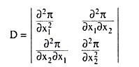
To alternate in sign starting from the negative. That is, the SOCs are:

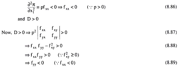
Therefore, the SOCs for profit-maximisation is given by (8.86) and (8.89).

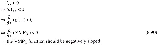
To interpret condition (8.86), let us note that

Similarly, condition (8.89)would give us

i.e., the VMP_Y function should be negatively sloped.

The SOCs imply, therefore, that the value of marginal product function of each input should be negatively sloped w.r.t. the input quantity.

Also, conditions (8.86), (8.88) and (8.89) require that the production function (8.21) of the firm should be strictly concave in the neighbourhood of a point at which the FOCs are satisfied with x, y ≥ 0, if such a point exists.