In this article we will discuss about:- 1. Introduction to Pareto Optimality 2. Efficiency in Production 3. Pareto Optimality in Production and Perfect Competition 4. Efficiency in Consumption or Exchange 5. Pareto Optimality in Consumption or Exchange and Perfect Competition 6. Pareto Optimality Conditions when the External Effects are Present and Other Details.
Contents:
- Introduction to Pareto Optimality
- Efficiency in Production
- Pareto Optimality in Production and Perfect Competition
- Efficiency in Consumption or Exchange
- Pareto Optimality in Consumption or Exchange and Perfect Competition
- Pareto Optimality Conditions when the External Effects are Present
- Efficiency in the Allocation of Factors among Commodities, or, Efficiency in Product-Mix or Composition of Output
- Pareto-Optimal Composition of Outputs and Perfect Competition
1. Introduction to Pareto Optimality:
ADVERTISEMENTS:
The welfare of a society depends, in the broadest sense, upon the satisfaction levels of all its consumers. But almost every change in the economic state of the society will have favourable effects on some members and unfavorable effects on others.
Evaluation of such a social change is impossible unless the economist is ready to go into interpersonal comparison of utility under some value judgement, which he may not be willing to do. Rather, he will be willing to evaluate such changes where at least one person has been better off and no one worse off.
The Italian economist Vilfredo Pareto (1848-1923) said that if a change in the economic state makes at least one individual better off without making anyone worse off, then the change is for the betterment of social welfare, i.e., the change is desirable. In that case, we say that the initial state was Pareto-non-optimal.
On the other hand, if a change makes no one better off and at least one worse off, implying that the change will make the society worse off, then, from the point of view of welfare, the initial economic state is Pareto-optimal.
ADVERTISEMENTS:
Therefore, the Pareto optimality criterion can be stated in this way:
A situation in which it is impossible to make any one better off without making someone worse off, is said to be Pareto optimal or Pareto-efficient.
Obviously, the concept of Pareto optimality avoids interpersonal comparison of utility. Since most government policies involve changes in the economic state, which benefit some people and bring discomforts to others, it is obvious that the concept of Pareto optimality is of limited applicability in the real world situations.
Pareto Optimality Conditions:
ADVERTISEMENTS:
For the attainment of Pareto-efficient situation in an economy, three marginal conditions must be satisfied.
These are:
(i) Marginal condition for efficiency in the allocation of factors among firms (efficiency in production);
(ii) Marginal condition for efficiency of distribution of commodities among consumers (efficiency in consumption); and
(iii) Marginal condition for efficiency in the allocation of factors among commodities (efficiency in product-mix or composition of output).
Assumption:
In order to derive these three marginal conditions for the attainment of Pareto optimality, we shall assume, for the sake of simplicity, that there are only two consumers (I and II), two factors of production (X1 and X2). and two commodities (Q1 and Q2), i.e., our model here would be a 2 x 2 x 2 model.
2. Efficiency in Production:
If we assume that the consumer goods are of “more is better” type and that external effects are absent in consumption, then an increment in the quantity produced of at least any one consumer good without a decrement in the quantity of any other, can lead to an improvement in utility level of at least one consumer without utility decrements for others.
ADVERTISEMENTS:
Therefore, Pareto optimality in production requires that the output level of each consumer good be at a maximum, given the output levels of all other consumer goods.
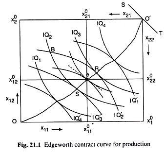
We may derive the marginal condition for Pareto-efficiency in production with the help of Fig. 21.1 which is called an Edge-worth box diagram. The dimensions of the rectangle in Fig. 21.1 represent the total available quantities, and x02, of the inputs X1 and X2 that would all be used to produce the consumer goods Q1 and Q2.
Any point in the box represents a particular allocation of the inputs over the production of the two goods.
ADVERTISEMENTS:
For example, if the allocation of the inputs is given by the point B, the quantities of X1 and X2 used in the production of good Q1 are measured by the coordinates of B with reference to the origin O, and the quantities of X1 and X2 used in the production of good Q2 are measured by the coordinates of point B with reference to the origin O’.
The isoquant (IQ) maps for goods Q, and Q2 are given in Fig. 21.1 with reference to the points of origin O and O’, respectively.
Now, the marginal condition for Pareto efficiency in production would be obtained if we maximise the output of good Q1 subject to a given output level of good Q2. Such maximisation would occur at a point of tangency between the IQs for the two goods.
For example, maximisation of output of Q1 subject to the quantity of Q2 as given by IQ3, would occur at the point of tangency S between the IQs for the goods. Similarly, maximisation of output of Q2 subject to the quantity of Qi as given by IQ3, would occur at the point of tangency R between the IQs for the two goods.
ADVERTISEMENTS:
However, at the point of tangency between the IQs for the two goods, we have numerical slope of IQ for good Q1 = numerical slope of IQ for good Q2
MRTSX1, X2 or, in the production of Q1 = MRTSX1,X2 in the production of Q2 (21.1)
Thus, the marginal condition for Pareto efficiency in production is given by (21.1) which states that the marginal rate of technical substitution (MRTS) between the two inputs should be the same in the production of the two goods.
It is obvious from above that the Pareto efficiency point in production must necessarily be a point of tangency between the IQs for the two goods. If we join all the points of tangency between the IQs for the two goods, by a curve, we would obtain what is called the Edge-worth contract curve for production which we would denote by CCP. The CCP would run from the point O to the point O’ in Fig. 21.1.
We have obtained then that all the points on the CCP are Pareto-efficient points in production. That is, if we are at some point on the CCP, then we are no longer able to effect by a change in the allocation of the inputs, an increase in the output of one of the goods without reducing the quantity of the other.
On the other hand, any point like B in Fig. 21.1, which does not lie on the CCP and which does not satisfy condition (21.1), is Pareto-non-optimal. At the point B, we are on IQ2 for good Q1 and on IQ’2 for good Q2.
ADVERTISEMENTS:
However, after a reallocation of the resources, if the economy reaches at some point on the CCP between R and S, then the quantities of both the goods would be larger, and if the economy reaches just at the point R or S, then the quantity of one of the goods would be larger and that of the other good would remain the same.
This shows that any point B that does not lie on the CCP, is Pareto-non-optimal, and, by a reallocation of the resources, if the economy is brought on to some point on the segment RS of the CCP, then at least one of the goods would be produced in a larger quantity, that of the other remaining the same.
We have seen that all the points on the CCP are Pareto-optimal. However, we cannot compare any two points, e.g., R and S, on the CCP because if the economy moves from S to R, the output of Q1 would increase and that of Q2 would decrease resulting in advantage for some people and disadvantage for some others, and since interpersonal comparison of utility is ruled out, we cannot compare the points R and S.
Mathematical Derivation of the Conditions:
We may also derive mathematically the marginal condition for Pareto efficiency in production.
Let us suppose that the production functions for the goods Q1 and Q2 are:
ADVERTISEMENTS:
q1 = q1 (x11, x12)
and q2 = q2 (x21, x22) (2.12)
where q1 and q2 are the quantities produced of goods Q1 and Q2, x11 and x12 are the quantities of inputs X1 and X2 used in the production of Q1, and x21 and x22 are the quantities of these inputs used in the production of good Q2.
Since the total available quantities of the two inputs are x01 and x02, we may write:
As per the requirements of Pareto optimality, the efficiency conditions may be derived if we maximise q1 as given by (21.2) subject to:
where q02 is any given quantity of good Q2.
The relevant Lagrange function for this constrained maximisation problem is:
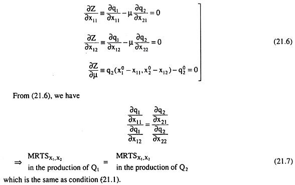
The first order or the necessary conditions for maximum q1 subject to q2 = q02 are:
Pareto efficiency condition (21.1) or (21.7) gives us that the available quantities of the two inputs, X1 and X2, should be allocated over the production of the two goods, Q1 and Q2, in such a way that the MRTS between the inputs may be the same in the production of the two goods.
ADVERTISEMENTS:
We may now see with the help of a simple example why condition (21.7) is necessary for Pareto efficiency in production. Let us suppose that in the production of Q1, MRTSX1,x2 = 2 and, in the production of Q2, MRTSX1,x2 = 1
i.e., the MRTS is not the same in the production of the two goods.
It follows from above that we can substitute 1 unit of X1 for 2 units of X2 in the production of Q1, and keep the output of Q1 constant. Similarly, we can substitute 1 unit of X1 for 1 unit of X2 in the production of Q2, and keep the output of Q2 constant. So, all we have to do is to take 1 unit of X1 out of the production of Q2 and use it in the production of Q1.
This releases 2 units of X2 from the production of Q1, 1 unit of which may be transferred to the production of Q2 to keep its output at the initial level. If we do all this, the output of Q1 and Q2 would remain unchanged, and yet we are left with an extra unit of X2. We can use this unit in the production of Q1 (or Q2) and get more of Q1 (or of Q2). Thus, one output is increased without reducing the other output.
The above example shows that if the MRTSX1, X2 in the production of the two goods are not equal, if MRTS in the production of Q2 is lower, say, than that in the production of Q1; then we have to take away the marginal unit of input X1 from the production of Q2 and transfer it to the production of Q1 where the MRTSX1,X2 is higher, and take away from the field the input X2, in exchange.
As we continue the process, the MRTS in the production of Q2 would rise as the quantity of X1 falls, and the MRTS in the production of Q1 would fall as the quantity of X1 increases, and, as we have seen, the allocation becomes better in the Pareto sense.
Therefore, if we are to reach the Pareto-efficient situation, we have to continue the process till the MRTS becomes equal in the production of the two goods. For when the MRTS in the production of both the goods becomes the same, no further reallocation will be able to increase the production of at least one of the goods without reducing the production of the other good.
To understand this, let us suppose that the MRTS between the two inputs are equal in the production of the two goods, and it is equal to 4. In that case, if we take away 1 unit of X, from the production of Q2, and transfer it to the production of Q1, the latter would release 4 units of X2 in exchange, so that the output level of Q1 might remain constant.
These 4 units of X2 should be transferred to the production of Q2 because there the MRTS is 4, and when 4 units of X2 are given to be used in the production of Q2 in exchange for 1 unit of X1, the output of Q2 would remain unchanged at the initial level.
Therefore, by means of a reallocation of the resources, we have not been able to increase the production of at least one of the goods. On the contrary, a reallocation of the inputs would keep the outputs of the two goods unchanged at their initial quantities.
3. Pareto Optimality in Production and Perfect Competition:
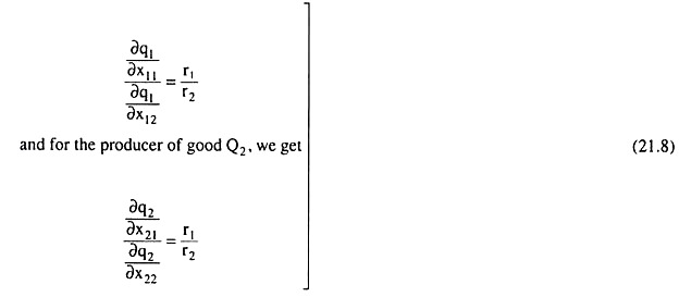
Pareto optimality in production is guaranteed under perfect competition. For, under perfect competition, the prices r1 and r2 of the two inputs, X1 and X2, are given to the firms that produce the goods Q1 and Q2, and each profit-maximising firm equates the MRTSX1,x2 to the ratio of the prices of the inputs.
That is, for the producer of Q1 we get:
From (21.8), we obtain:
MRTSx1, x2 in the production of Q1 = MRTSx1,x2 in the production of Q2 (21.9)
Since condition (21.9) is the same as condition (21.7), Pareto efficiency in production is a certainty under perfect competition.
We may now obtain a graphical solution of equation (21.7) or (21.9) for the allocation of inputs X1 and X2 over the production of goods Q1 and Q2 and for the quantities produced of Q1 and Q2. The satisfaction of the marginal condition (21.7) or (21.9) is guaranteed under perfect competition.
Let us suppose that in the competitive markets the prices of the inputs are given to be r1 and r2. Let us now draw a straight line ST of slope – r1/r2 through the point O’ in Fig. 21.1, and pick up the point e on the contract curve for production (CCP) where the common slope of the isoquants has been equal to the slope of the line ST. That is, at the point e, we have numerical slopes of the IQs of two individuals = the numerical slope of the line ST = r1/r2
That is, at the point e in Fig. 21.1, the marginal condition for efficiency of production has been satisfied. At this point quantities of the two inputs, x011 and x021 would be used in the production of Q1 and these quantities, when substituted in the production function for Q1, would give us the output quantity of Similarly, quantities of the two inputs, x021 and x022, would be used in the production of Q2 and the output here would be q02.
4. Efficiency in Consumption or Exchange:
A distribution of the given quantities of the two commodities Q1 and Q2 among two consumers I and II is said to be Pareto-efficient if it is impossible, by a redistribution of these goods, to increase the utility of one individual without 0 reducing the utility of the other.
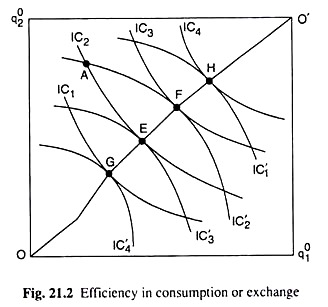
The marginal condition for efficiency in consumption or exchange can be derived with the help of the Edgeworth box diagram given in Fig. 21.2. The dimensions of the rectangle in Fig. 21.2 represent the total available quantities, q01 and q02, of the two goods in a pure- exchange economy.
Any point in the box represents a particular distribution of the commodities between the two consumers. For example, if the distribution of commodities is given by point A, the quantities of Q1 and Q2 consumed by consumer I are measured by the coordinates of A with respect to the origin O and the quantities of the two goods consumed by II are measured by the coordinates of A w.r.t. the origin O’.
The indifference map of consumer I has been given w.r.t. the origin O and that of II has been given w.r.t. the origin O’.
Now, the marginal condition for Pareto efficiency in consumption or exchange would be obtained if we maximise the utility level of consumer I or II subject to the given utility level of consumer II or I. Such maximisation would occur at a point of tangency between the indifference curves (ICs) of the two consumers. For example, maximisation of utility of consumer I subject to the utility level of II as given by IC1 of consumer II, would occur at the point of tangency, E, between the ICs of two consumers.
Similarly, maximisation of utility of consumer II subject to the utility level of I as given by IC3 of consumer I would occur at the point of tangency, F, between the ICs of the two consumers. It may be added, therefore, that the exchange equilibrium is not unique.
Now, at the point of tangency between the ICs of the two consumers, we have numerical slope of IC of consumer I = numerical slope of IC of consumer II
=> MRSQ1,Q2 of consumer I = MRSQ1,Q2 of consumer II (21.11)
Thus, the marginal condition for Pareto efficiency in consumption is given by (21.11). It is obvious from above that any point of tangency between the ICs of two consumers is a Pareto efficiency point. If we join all such points of tangency by a curve in Fig. 21.2, we obtain what is known as the Edgeworth contract curve for consumption or Exchange (CCC or CCE), which would run from the point O to the point O’.
Therefore, all the points on the contract curve at which (21.11) is satisfied, are Pareto-efficient points in consumption. For, if we are at some point on the contract curve, in Fig. (21.2), we are not able to effect, by a change in the distribution of the goods, an improvement in the utility of one consumer without reducing the utility of the other.
Therefore, let us note again that the point of Pareto efficiency in exchange is not unique. On the other hand, any point like A, which does not lie on the contract curve and which does not satisfy (21.11), is Pareto-non-optimal. At the point, A, consumer I is on his IC2 and consumer II is on his IC2.
However, after a redistribution of the commodities, if the consumers are brought at some point on the contract curve between E and F, then both the consumers would benefit for both of them would reach now higher ICs, and if they are brought just at the point E or F, then one of them will benefit, while the utility level of the other will remain the same.
This shows that any point A, which does not lie on the CCE, is Pareto-non-optimal and by a redistribution of the commodities, if we bring the consumers on to the EF segment of the CCE, then at least one of them would benefit, the utility level of the other remaining the same.
We have seen that all points on the contract curve are Pareto-efficient. However, we cannot compare the points on the contract curve because that will involve interpersonal comparison of utility, which is not possible without an explicit value judgement.
Mathematical Derivation of the Conditions:
We may also derive mathematically the marginal condition for Pareto efficiency in consumption, or, Exchange. Let us suppose that the utility functions of the two consumers I and II are respectively,
u1 =u1 (q21, q12)
and u2 = u2 (q21, q22) (21.12)
where q11 and q12 are the quantities of Q1 and Q2 consumed by consumer I and q21 and q22 are the quantities of the two goods consumed by individual II.
If and q2 are the given quantities of the two goods, then we have:
q11 +q21 =q01
and q12+q22=q02 (21.13)
It is evident from (21.12) that the utility level of each consumer depends only upon the quantities consumed by him and not upon the quantities consumed by the other. That is, it has been assumed here that external effects are absent.
Pareto-efficiency in consumption implies that u1 is maximised subject to a given u2 = u02, or, the other way round. Let us then form the relevant Lagrange function, V, for the constrained maximisation of u1 as
V = u1 (q11,q12) + λ[u2(q2(q21, q22)-u02] (21.14)
where λ is the Lagrange multiplier.
Now, the first-order conditions for the constrained maximisation of u1 subject to u2 = u02 are:
Pareto-efficiency condition (21.11) or (21.16) gives us that the given quantities of the two goods should be distributed among the two consumers in such a way that the MRS between the goods may be the same for the two consumers.
We may now see with the help of a simple example why condition (21.11) is necessary for Pareto efficiency in consumption.
Let us suppose that:
for individual I, => MRSQ1,Q2 = 2 and
for individual II, => MRSQ1,Q2 = 1
i.e., the MRS is not the same for the two individuals.
This means that individual I is willing to exchange 2 units of Q2 for getting 1 unit of Q1 and individual II is willing to exchange 1 unit of Q2 for getting 1 unit of Qi. In such a case, where the MRS is not the same for the two individuals, we may redistribute the goods to make at least one of them better off without making the other consumer worse off.
What we have to do here is to take away 1 unit of Q1 from consumer II and give it to I who will give us 2 units of Q2 in exchange. Now we give one of these units to B to keep his utility level constant—he wants to have 1 unit Q2 for giving up 1 unit of Q1.
But we have now 1 unit of Q2 left. We can give it to either I or II, and thus make either I or II better off without making the other person worse off. Thus, the initial allocation was not efficient.
The above example shows us that if the MRS of the two individuals are not equal, if the MRS of II is lower, say, than that of I, then we have to take away the marginal unit of good Q, from individual II and give it to I whose MRS is higher, and take away from him good Q2 in exchange.
As we continue the process, the MRS of II would rise as the quantity of Q1 with him decreases and the MRS of I would decrease as the quantity of Q1 with him increases, and, as we have seen, the distribution becomes better in the Pareto sense. Therefore, if we are to reach the Pareto-efficient situation, we have to continue the process till MRS of the two persons become equal.
For when the MRS of the two persons are equal, no further redistribution will be able to do good to at least one of them without harming the other. To understand this, let us suppose that MRS of both the persons are equal, and it is equal to 4.
In that case, if we take away 1 unit of Q1 from consumer II and give it to consumer I, the latter would give us 4 units of Q2 in exchange in order to keep his utility level intact. If we now give these 4 units of to individual II, his utility would assume the initial level. That is, by means of a redistribution of the goods, we have not been able to improve the utility level of at least one of the persons. On the contrary, a redistribution of the goods would keep the individuals on their initial utility levels.
5. Pareto Optimality in Consumption or Exchange and Perfect Competition:
It can be easily shown that Pareto optimality in consumption is automatically achieved under perfect competition. For under perfect competition, the prices P1 and P2 of the two goods are given to the consumers, and each utility-maximising consumer equates his MRS of Q1 for Q2 to the ratio of the prices of the goods.
That is, for consumer I, we get:
which is nothing but the Pareto-efficiency condition (21.16) or (21.11).
Thus, perfect competition guarantees Pareto-efficiency in the distribution of commodities among the consumers.
6. Pareto Optimality Conditions when the External Effects are Present:
The marginal condition for a Pareto-efficient distribution of given amounts of two goods (Q1 and Q2) between the two individuals (I and II) as given by (21.18) has been obtained on the basis of the assumption that externalities in consumption are absent.
We shall now see that if the external effects are present, the Pareto optimality condition in consumption would generally be different from the marginal condition (21.18).
Let us assume that the external effects are present in consumption in the sense that the utility level of one consumer depends also on the consumption of another.
Let us assume that the two consumers’ utility functions are given by:
Pareto optimality will be achieved if u1 is maximum subject to a given level of u2 = u02.
In order to derive the conditions for this constrained maximisation, we have to form the Lagrange function:
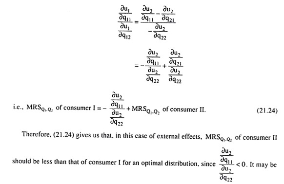
Equation (21.23) is the necessary’ condition for Pareto optimality in consumption when external effects are present. It generally differs from the Pareto optimality marginal condition as given by (21.18) or (21.16) or (21.11).
Perfect completion guarantees the attainment of (21.11) but not of (21.23). It is evident from (21.23) that if the external effects were absent, we would have ∂u1/∂q21, ∂u1/∂q22, ∂u1/∂q11 and ∂u2/∂q12, all equal to zero, and then (21.23) would have reduced to (21.11).
Since we have assumed here that the partial derivatives of the utility functions are functions of all variables, viz., q11, q12, q21 and q22, the optimum position of each consumer depends upon the consumption level of the other.
For example, if we assume that the only external effect present in the two-consumer model is ∂u2/∂q11 <; 0, then equation (21,23) becomes:
intuitively understood why this is so. If consumer I’s consumption of Q1 increases, then the utility level of consumer II declines. This implies that the marginal significance of Q1 to consumer II is relatively large, which, again, implies that the MRSQ1,Q2 of consumer II should be smaller at the state of optimal distribution of the goods.
For, at this distribution as compared with the MRS-equating distribution, the quantity of Q1 possessed by consumer II would be larger than that possessed by consumer I.
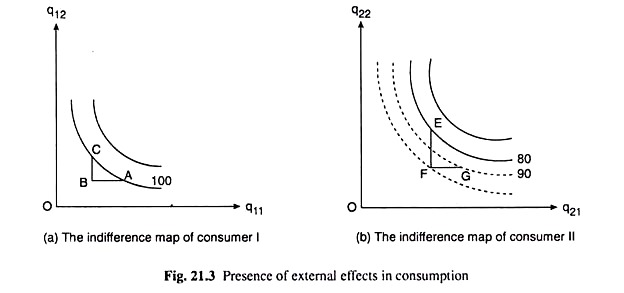
It can be shown diagrammatically with the help of Fig. 21.3 that condition (21.16) does not necessarily ensure Pareto optimality in the presence of external effects. Figures 21.3(a) and 21.3(b) give us the indifference map of consumers I and II, respectively. Let us assume that initially, consumer I consumes the combination A and consumer II consumes the combination E.
The MRSQ1,Q2 of the two consumers are equal at their utility maximising points, given the prices of the goods. Let us now assume that there are no external effects for consumer I, i.e., I’s utility level is not affected by the consumption of II.
Although, consumer II’s utility level is affected by the consumption of consumer I. Let us suppose, as we have done above, that as I consumes more of Q1, II’s utility level declines, i.e., ∂u2/∂q11 < 0. This is the external effect present here.
Now, in Fig. 21.3(b), consumer II’s indifference curves (solid ones) have been drawn on the assumption that I’s consumption is given by combination A. In their individual equilibrium situations, consumer I’s utility index is 100 and that of II is 80.
Let us now redistribute the commodities between the two individuals such that their aggregate quantities remain unchanged and I moves to point C having less of Q1 and more of Q2 and II moves to point G having more of Q1 and less of Q2 (AB = FG and BC = EF). The utility level of consumer I has not changed because of this redistribution—he remains on the same IC.
However, since consumer I’s consumption of Q1 has decreased, consumer II’s preference- indifference pattern would be affected. His new ICs are given by the dotted curves. Also, at the point G, consumer II’s utility level has increased to 90 since I is now consuming less of Q1.
Therefore, by means of the redistribution, we have been able to raise II’s utility level, I’s level remaining constant. That is, the initial equilibrium positions at A and E where the MRS of the consumers had been equal, were Pareto non-optimal. Therefore, we have seen that equality of MRS of the two consumers does not ensure Pareto optimality.
In the present equilibrium situations, the MRS of consumer I has increased since he has moved north-westward along the same IC, and the MRS of II has decreased since he has moved southeastward, not along the same IC, but along an almost parallel IC.
That is, if the said external effect is present, consumer II’s MRS would be less than that of consumer I. This result we have already obtained in the mathematical analysis given above.
7. Efficiency in the Allocation of Factors among Commodities, or, Efficiency in Product-Mix or Composition of Output:
A composition of output or product-mix is Pareto-efficient if it is impossible to increase the utility of one individual without reducing the utility of the other by reallocating the factors among the commodities, leading to a different product-mix.
The marginal condition for a Pareto-efficient product-mix states that the marginal rate of product transformation (MRPT) of Q2 into Q1 must be the same as the marginal rate of substitution (MRS) of Q1 for Q2, for each consumer.
Here, the MRPT of Q2 into Q1 is equal to the quantity by which the production of Q2 has to be reduced in order to produce one more (or the marginal) unit of Q1 and, as such, it is equal to the numerical slope of the economy’s production possibility curve or frontier (PPC or PPF).
An economy’s PPC passes through all the combinations of the two goods (Q1 and Q2) that the available quantities of the two inputs (X1 and X2) can produce Pareto-efficiently. That is, any combination of the two goods that lie on the PPC gives us the maximum quantity of Q1 that can be produced subject to the production of a given quantity of Q2, or, the maximum of Q2 subject to a given quantity of Q1.
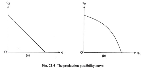
In other words, the combinations of the two goods that lie on the PPC are those that lie on the Edge-worth contract curve for production (CCP) [Fig. 21.1]. That is, there is a one-to-one correspondence between the points on the CCP and those on the PPC. Since, as we move along the CCP, the quantity of one of the goods increases and that of the other decreases, the slope of the PPC would be negative.
Also, as more and more inputs are removed from the production of Q2 and are engaged in the production of Q1, Q2 may be transformed into Q1 at a constant rate in which case the PPC would be a negatively sloped straight line with its numerical slope or MRPT being a constant, or, which is more likely, Q2 may be transformed into Q1 at an increasing rate owing to the law of diminishing marginal product, in which case the PPC would be concave to the origin with its numerical slope or MRPT rising as Q1 increases and Q2 diminishes, i.e., as we move southeastward along the curve. We have shown these two types of PPC in Fig. 21.4.
Now, since the MRPT shows the rate at which a good can be transformed into another in production and the MRS shows the rate at which the consumers are willing to exchange one good for another, the Pareto-efficient product-mix cannot be obtained unless the two rates are equal. Only then the production sector’s plans may be consistent with the household sector’s plans, and the two are in equilibrium.
We may illustrate the argument with the help of a simple numerical example. Let us assume that at any particular product composition, the MRPT is 7, i.e., 7 units of Q2 can be transformed into 1 unit of Q1.
On the other hand, at this product composition, the MRS for each consumer is, say, 3. That is, for substituting an additional (or the marginal) unit of Q1, each consumer is willing to forego 3 units of Q2 so that his utility level might remain constant.
To improve the welfare situation, what we may do in this case is: we may take away from each consumer 1 unit of Q1 and in its place we may have 7 units of Q2 and then, out of these 7 units, we may give 3 units to the consumer to compensate for his loss of 1 unit of Q1. We are then left with 4 units of Q2 for each consumer.
If their number is 2, then we are left with 8 units of Q2 some of which we may give to consumer I and some to consumer II. Thus the utility level of both the consumers would increase. This shows us that the initial situation of MRPT ≠ MRS was Pareto-non-optimal.
Now, as we take away Q1 from each consumer, his MRSQ1,Q2 would increase (from 3) and as we move northwestward along the PPC curve to have Q2 in its place, the MRPT would decrease (from 7). We have to continue the process unless at some product composition MRPT becomes equal to MRS.
Therefore, the marginal condition for the Pareto-efficient product-mix gives us that the MRPT between the products should be equal to the MRS of each consumer. It may very well be seen that once these two become equal, no improvement in welfare can be achieved by any further change in product composition.
For example, if both MRPT and MRS are equal to 5, say, then, if we take away 1 unit of Q1 from each consumer, 5 more units of Q2 would be obtained in its place, and all of these 5 units would have to be given to the consumer to compensate for his loss of 1 unit of Q1—to keep him on his initial utility level. Thus, nothing would be available for any improvement.
On the basis of the above analysis, we may write the marginal condition for the Pareto- efficient product-mix or composition of output as
MRPTQ2 into Q1 = MRSQ1,Q2 of consumer I = MRSQ1,Q2 of consumer II (21.25)
8. Pareto-Optimal Composition of Outputs and Perfect Competition:
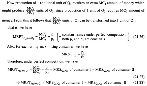
Like the other two marginal conditions, the third marginal condition of Pareto-efficient composition of output is also guaranteed by perfect competition, where the prices p1 and p2 of the goods Q1 and Q2, are given to the two firms and two consumers.
Also, in profit-maximising equilibrium under perfect competition, we have the marginal cost of production (MC1) of Q1 equal to pi and the marginal cost of production (MC2) of Q2 equal to p2 (i.e., p1 = MQ and P2 = MC2).
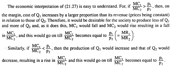
We have seen above that the Pareto-efficient product-mix cannot be obtained unless the MRPT of Q2 into Q1 and the MRS of Q1 for Q2 for each consumer are equal, and that this condition is guaranteed under perfect competition. We may now see graphically how eqn. (21.28) can be solved for the combination of the two goods that would make the production sector’s plans consistent with the household sector’s plans.
We have obtained, therefore, that the equilibrium commodity combination for our society consisting of two profit-maximising firms and with given quantities (x01 and x02) of two inputs, is the one where the condition given by equation (21.27) or equation (21.28) is satisfied.
We might remember at this point that the PPC passes through the commodity combinations implicit at the points on Edgeworth contract curve for production (CCP), i.e., these commodity combinations on the CCP have been mapped into the PPC, or, there is a one-to-one correspondence between these commodity combinations implicit at the points on the CCP and those lying on the PPC.
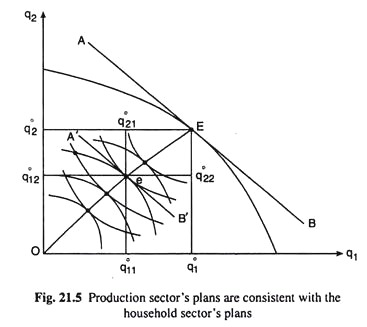
(21.27) gives us that the point where the condition for equilibrium commodity combination is satisfied is the point of tangency between the PPC curve and line of slope –p1/p2. In Fig. 21.5, AB is this line, say, and it has touched the PPC curve at the point E. Therefore, the society’s equilibrium production point is the point E, and it should produce q01 and q02 of the two commodities.
We may now come to the distribution of the goods between the two consumers, I and II. They have to be so distributed that the Pareto-efficiency in consumption is achieved, i.e., the marginal condition for such efficiency is satisfied.
As we know, this marginal condition is:
We also know that the satisfaction of this condition is guaranteed under perfect competition, since both of them would be equal to p1/p2 which is given and constant:
In Fig. 21.5, the Pareto-efficient distribution of the goods is obtained at the point e on the Edgeworth contract curve for consumption (CCC), for, at this point, both the indifference curves (ICs) of the two consumers have touched the line A’B’ which is parallel to the line AB.
That is, in order to obtain the Pareto-efficient distribution of the goods, we have to find out the point (like e) on the Edgeworth CCC at which the numerical slopes of the ICs of the two consumers are equal to p1/p2 which is here the numerical slope of the line AB.
To be more specific, as the solution of eqn. (21.26), we have obtained the economy’s production of the two goods to be E(q01q02) and by solving (21.17), we would obtain the distribution of these quantities between the two consumers (at the point e) to be (q011, q012) for the first consumer and (q021,q022) for the second consumer.
