Theory of Determination of National Income| Economy

The theory of determination of national income is concerned with finding out the equilibrium level of national income, i.e., the level of national income at which the purchas­ing and production plans of the economy are synchro­nised. This occurs at the point of the intersection of the ag­gregate demand (C + I) sched­ule and the aggregate supply (C + S) schedule. This is shown by point A in Fig. 3.

Income levels above point G cannot be maintained because total spending is insufficient to buy up all the output being produced. Business firms find themselves with unsold stocks and are thus forced to cut back production. In contrast, at income levels below point E aggregate expenditure exceeds available output. Now, business firms find that they can sell their entire output. So, they are encouraged to produce more to meet the additional demand that exists.

National income equilibrium is also reached at the point where total injections exactly equal leakages. In a closed economy without government, the only injection is autonomous investment and the only leakage is saving.

Thus, the leakages-injections approach to national income determination also goes by the name saving-investment approach. In the circular flow of national income model, income – consumption + leakages = C + S and spending (expenditure) = consumption + injections = C + I.

See Fig. 3. Here, equilibrium is achieved where leakages = injections, i.e., point £ which is the same as point E in the income and expenditure schedules in Fig. 1. If leakages exceed injections then total expenditure will fall, resulting in a contraction of income and output. Conversely, if injections exceeds leak­ages, then total expenditure will rise, resulting in an increase in income and output. Only when injections and leakages are equal national income and output will remain the same.

The equilibrium level of national income will change if there is a shift in the aggregate expen­diture schedule. For example, if aggregate demand rises from AE₁ to AE₂ due to an increase in investment spending, there will be an increase in the equilibrium level of national income from Y_E to Y_F.

Alternatively, the equilib­rium level of national income will change if there is a shift in either the leakages or injections sched­ules. For example, an increase in investment spending will shift the investment demand schedule upward from I₁ to I₂, resulting to an increase in the equilibrium level of income from Y₁ to Y₂ as shown in Fig. 4.

The Multiplier Effect:

Keynes also pointed out that an act of autonomous spending will have a multiplier effect. It was he who first introduced the concept of investment multiplier to show the relation between any change in autonomous spend­ing (such as investment) and the resulting change in national income. In fact, the multiplier is the number by which the change in autonomous investment has to be multiplied to find out the resulting change in equilibrium national income.

In other words, it is the ratio of an induced change in the equilib­rium level of national income to an initial change in the level of investment spending. ‘The multiplier effect’ denotes “the phenomenon whereby some initial increase (or decrease) in the rate of spending will bring about a more than proportionate increase (or decrease) in national income”.

We have to note two important points in this context:

Firstly, equilibrium income is not necessarily the level of income at which full employment is attained. In fact, an equilibrium level of income can occur at any level of economic activity. According to Keynes, full employment equilibrium is a special case where aggregate desired expenditure is exactly equal to potential output (GNP), leaving neither an inflationary nor a deflationary gap. For example, aggregate demand curve A₂ in Fig. 2 repre­sents full employment equilibrium where F corresponds with full employ­ment (potential output).

The second point to note here is that according to Keynes any act of autonomous spending will have a multiplier effect. In a two-sector model, the only item of autonomous spending is investment which is independent of income. And Keynes developed the theory of multiplier to denote the phenomenon whereby some initial increase in the rate of spending (autono­mous investment) will bring about a more than proportionate increase in national income. Thus, we can write

Δ Y = m (ΔI) … (1)

where, ΔY is the change in national income, Δ I is the initial change in investment spending and m is the investment multiplier.

We can also express equation (1) in the following form:

m = ΔY/ΔI … (2)

Thus, the multiplier is the ratio of the induced change in the equilibrium level of national income to an initial change in the level of spending.

Two features:

There are two important features of the multiplier process, (a) First, it is a cumulative process rather than an instantaneous effect. Thus, it is best viewed in terms of a series of successive ’rounds’ of additions to income, (b) Secondly, the numerical value of the multiplier depends on the fraction (proportion) of extra income that is spent on consumption (i.e., the marginal propensity to consume) at each successive round.

For simplicity, let us assume that all income is either consumed or saved. In fact, income is partly spent on consumption goods and partly saved. So the sum of MPC and MPS = 1.

The value of the multiplier (m) is then given by the formula:

m = 1/1 – MPC = 1/1 – MPS … (3)

The Multiplier and the Marginal Propensities to Consume and Save:

Since the multiplier is the reciprocal of MPS, its value depends on MPC. The larger the MPC, the larger is the multiplier.

Aggregate expenditure and national income (Y) change because con­sumption expenditure (C) and investment (I) changes. The changes in Y equals the change in C plus the change in I, i.e., ΔY = ΔC + ΔI.

But the change in consumption expenditure is determined by the change in y and the MPC. It is ΔC = MPC x ΔY.

Now, combining the two factors we get: ΔY = MPC x ΔY x ΔI. Now, solving for the change in Y as (1 – MPC) x ΔY = ΔI and rearranging, we get:

ΔY = ΔI/ (1 – MPC) … (4). The multiplier is m = ΔY/ΔI. So, dividing both sides of equation (4) by the change in investment (ΔI), we get:

m = ΔY/ΔI = 1/ (1 – MPC) = 1/MPS

Since, the MPS is a fraction — a number lying between 0 and 1 — the multiplier is greater than 1.

The larger the proportion of income which is spent on consumption goods, the larger the value of the multiplier. Thus if, MPC – 0.90 and MPS = 0.10 the value of the multiplier is 10. If MPC = 0.75 and MPS = 0.25 the value of the multiplier is 4.

Why is the multiplier related to MPS even if saving is a leakage from the circular flow of income? The answer is that if investment increases by a certain amount, say, Rs. 100 crores, and MPS is 1/5, income has to rise 5 times the increase in autonomous investment (i.e., Rs. 500 crores) so that the additional saving generated (1/5 of Rs. 500 crores or Rs. 100 crores) is just sufficient offset the additional investment and the economy is enabled to re-achieve equilibrium at a higher level of saving and investment.

In each round a proportion of extra income created is saved and is thus withdrawn from the circular flow. So, the proportion that leaks from the circular flow does not pass on as additional consumption spending in the next round. When the cumulative total of these leakages (savings) is exactly equal to the initial increase in spending, the multiplier process comes to a halt. And the economy reaches a new equilibrium.

Fig. 5 shows the multiplier effect graphically. Starting at the national income level OY₁ if aggregate expenditure increases from AE₁ to AE₂ then the initial injection of extra spending AB would lead to an increase of output (income) by Y₁Y₂.

This additional income would induce yet another round of consumption spending (CD) which would, in its turn, in­crease output and income by Y₂Y₃. This extra income would again induce more spending (EF) which would, in turn, in­crease output and income again by Y₃Y₄ and SO the process would continue for sometimes. The whole process would ultimately come to a halt when the new equilib­rium level of income Y_e is reached.

An example:

Let us consider a simple example. Let there be an increase of investment of Rs. 1000 crores. If this causes an increase in output of Rs. 3000 crores, then the multiplier is 3. If, instead, the resulting increase in output were Rs. 4000 crores, then the multiplier would be 4. In the words of Samuelson, “The multiplier is the number by which the change in invest­ment must be multiplied in order to determine the resulting change in total output”.

Since in an interdependent economy, one man’s expenditure is another man’s income, when Mr. X hires unemployed resources and spends Rs. 1,000 to build a writing table, there will be a secondary expansion of national income and production over and above his primary investment. Let us see why and how this happens.

Mr. X’s carpenters and lumber producers will get an extra Rs. 1,000 of income. If they all have a marginal propensity to consume of 2/3, they will now spend Rs. 666.67 on new consumption goods like food and clothing.

The producers of these goods will now have extra income of the same amount. If their MPC is also 2/3, they, in turn, will spend Rs. 444.44, or 2/3 of Rs. 666.67 (or 2/3 of Rs. 1,000). So, the process will go on with each round of spending being 2/3 of the previous round.

Thus, a whole endless chain of secondary consumption responding is set in motion by X’s primary Rs. 1,000 on investment spending. But this process cannot continue for long. It will ultimately come to a halt when the last increase in consumption spending is not sufficient to generate fresh income. And it ultimately adds up to a finite amount.

In our example the total increase in spending will be:

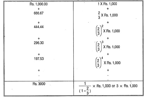
This simply shows that when MPC is 2/3, the multiplier is 3, consisting of the 1 of primary investment plus 2 extra of secondary consumption responding.

The multiplier be 4 if the MPC where 3/4, for the reason that l + 3/4 + (3/4)⁴ .. + finally adds up to 4. If the MPC were 1/2, the multiplier would be 2.

There is a close relation between the propensity to consume and the invest­ment multiplier. The size of the multiplier thus depends upon how large tire MPC is; or it can be expressed in terms of the MPS. If the MPS were 1/4, the multiplier would be 4. If the MPS were 1/5, the multiplier would be 5. If the MPS were 1/2 the multiplier would be 2.

In fact, the simple multiplier is always the “reciprocal” of the marginal propensity to save. So it can be expressed as 1/ (1 – MPC)

Our simple multiplier formula is

Change in output = 1/MPS × Change m investment

= 1/ (1 – MPC) × Change in investment

The multiplier effect can be illustrated in terms of savings-investment approach. A look at Figure 2 can confirm this. Our old investment schedule II is shifted upward by Rs.100 crores to new level I’I’, say, due to a rise in marginal efficiency of capital. The new intersection point is E’. And the increase in income is exactly three times as much as the increase in invest­ment.

This is so because an MPS of only 1/3 means a relatively flat saving schedule, such as SS. In this diagram the horizontal output distance is three times as great as the upward shift in the investment schedule, the excess being the secondary “consumption responding”.

What is happening is that output must rise enough to induce a volume of desired saving that equals the new investment. With an MPS of 1/3, income has to rise by how much in order to bring out Rs. 100 crores of new saving to match exactly the new investment?

Only one answer is possible. By exactly Rs. 300 crores.