In this essay we will discuss about Monopolistic Competition. After reading this essay you will learn about: 1. Meaning of Monopolistic Competition 2. Price Determination of a Firm under Monopolistic Competition 3. Chamberlin’s Group Equilibrium 4. Theory of Excess Capacity 5. Selling Costs 6. Wastes of Monopolistic Competition.
Contents:
- Essay on the Meaning of Monopolistic Competition
- Essay on the Price Determination of a Firm under Monopolistic Competition
- Essay on Chamberlin’s Group Equilibrium
- Essay on Theory of Excess Capacity
- Essay on the Selling Costs
- Essay on Wastes of Monopolistic Competition
Essay # 1. Meaning of Monopolistic Competition:
Monopolistic competition refers to a market situation where there are many firms selling a differentiated product. “There is competition which is keen, though not perfect, among many firms making very similar products.”
No firm can have any perceptible influence on the price-output policies of the other sellers nor can it be influenced much by their actions. According to Salvatore, “Monopolistic competition refers to the market organisation in which there are many firms selling closely related but not identical commodities.”
ADVERTISEMENTS:
Products are close substitutes with a high cross-elasticity and not perfect substitutes, Tata, Lipton, etc. tea; Hamam, Lux etc. soap; Pepsi, Coca Cola, etc. cold drinks are examples of product differentiation. Under monopolistic competition, no single firm controls more than a small portion of the total output of a product.
As the products are close substitutes, a reduction in the price of a product will increase the sales of the firm but it will have little effect on the price-output conditions of other firms, each will lose only a few of its customers. Likewise, an increase in its price will reduce its demand substantially but each of its rivals will attract only a few of its customers.
Therefore, the demand curve (average revenue curve) of a firm under monopolistic competition slopes downward to the right. It is elastic but not perfectly elastic within a relevant range of price at which he can sell any amount.
It means that it has some control over price due to product differentiation and there are price differentials between firms. Despite this, the slope of the demand curve is determined by the general level of the market price for the differentiated product.
ADVERTISEMENTS:
In so far as it exercises some control over price, it resembles monopoly and since its demand curve is affected by market conditions, it resembles pure competition. Such a situation is, therefore, characterised as monopolistic competition.
Essay # 2. Price Determination of a Firm under Monopolistic Competition:
The equilibrium of the firm under monopolistic competition follows the usual analysis in the short-run and long-run.
(A) Short-Run Equilibrium Assumptions:
The short-run analysis of the firm under monopolistic competition is based on the following assumptions:
(1) The number of sellers is large and they act independently of each other. Each is a monopolist in his own sphere;
ADVERTISEMENTS:
(2) The product of each seller is differentiated from the other products;
(3) The firm has a determinate demand curve (AR) which is elastic;
(4) The factor-services are in perfectly elastic supply for the production of the product in question;
(5) The short-run cost curves of each firm differ from each other; and
(6) No new firms enter the industry.
Explanation:
Given these assumptions, each firm fixes such price and output which maximises its profits. The equilibrium price and output is determined at a point where the short-run marginal cost curve (SMC) cuts the marginal revenue (MR) curve from below.
Since costs differ in the short-run, a firm with lower unit costs will be earning only normal profits. In case, it is able to cover just the average variable cost, it incurs losses.
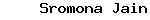
In Figure 1 (A) the short-run marginal cost curve (SMC) cuts the MR curve at E. This equilibrium point establishes the price QA (=OP) and output OQ. As a result, the firm earns supernormal profits represented by the shaded area PABC.
ADVERTISEMENTS:
Figure 1 (B) indicates the same equilibrium point of price and output. But in this case the firm just covers the short-run average unit cost as represented by the tangency of demand curve D and the short-run average unit cost curve SAC at A. It earns normal profits.
Figure 1 (C) shows a situation where the firm is not able to cover its short-run average unit cost and therefore incurs losses. Price set by the equality of SMC and MR curves is QA which covers only the average variable cost.
The tangency of the demand curve D and the average variable cost curve A VC at A makes it a shut-down point. If the firm lowers the price below QA, it will have to stop further production. However at this price, the firm will incur losses equal to the area CBAP during the short-run in the hope of lowering its costs in the long-run.
ADVERTISEMENTS:
It is not essential that during the short-run all firms charge identical prices and produce the same quantity as we have shown above. This is to simplify our geometrical presentation. There being product differentiation, identity of prices and quantities cannot be expected.
Each firm acts in accordance with its own short-run costs and equates its SMC curve with the MR curve. However, this does not mean that the firm fixes a very different price from the other producers. Since its product has close substitutes, its price will have to approximate to the prices of the other firms producing a similar product.
(B) Long-Run Equilibrium:
In the long-run, there is entry and exit of firms in a monopolistic competitive industry as under pure competition, the adjustment process will ultimately lead to the existence of only normal profits. This is a realistic assumption for in the long-run no firm can earn either super-normal profits or incur losses because each produces a similar product.
If firms in the monopolistic competitive industry are earning super-normal profits, new firms will be attracted into the group. With the entry of new firms, the existing market is divided among more sellers so that each firm will sell lesser quantities of the product than before. As a result, the demand curves faced by individual firms shift down to the left. At the same time.
ADVERTISEMENTS:
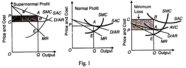
The entry of new firms will increase the demand and hence the price of factor-services will rise which will shift the cost curves of individual firms upward. This two- way adjustment process of lowering the demand curve and raising the cost curves will squeeze out supernormal profits. Thus, each firm will be earning only normal profits in the long-run, as shown in Figure 2.
In the figure, all firms are in the long-run equilibrium at point E where (1) LMC = MR and (2) LMC cuts MR from below, and the LAC curve is tangent to the D/AR curve at point A. Since price QA = LAC at points, each firm is earning normal profits and no firm has the tendency to enter or leave the industry.
This long-run equilibrium analysis under monopolistic competition reveals that each firm and the entire industry will not produce optimum output. There will always be excess capacity. For the firms are not in a position to operate their plants to the maximum capacity and thus enjoy the economies of large scale production fully.
It is evident from Figure 2 where the point of tangency between the demand curve D/AR and the LAC curve is not at the lowest level L. Rather, L is to the right of the point of tangency A. This is because the demand curve D/AR is not horizontal but slopes downward to the right. Thus each firm under monopolistic competition has unutilized capacity even in the long-run.
Essay # 3. Chamberlin’s Group Equilibrium:
Concept of Industry and Group:
Group equilibrium relates to the equilibrium of the “industry” under a monopolistic competitive market. The word “industry” refers to all the firms producing a homogeneous product. But under monopolistic competition the product is differentiated.
ADVERTISEMENTS:
Therefore, there is no “industry” but only a “group” of firms producing a similar product. Each firm produces a distinct product and is itself an industry. Chamberlin lumps together firms producing very closely related products and calls them product groups.
So in defining an industry, Chamberlin lumps together firms in such product groups as cars, cigarettes, breweries, etc. According to Chamberlin, “Each producer within the group is a monopolist, yet his market is interwoven with those of his competitors, and he is no longer to be isolated from them.”
In the product group, the demand for each product has high cross elasticity so that when the price of other products in the group changes, it shifts the demand curve.
Theory of Group Equilibrium:
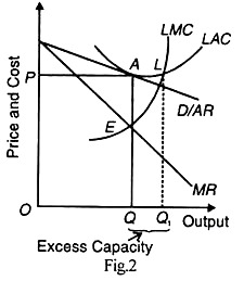
Chamberlin develops his theory of long-run group equilibrium by means of two demand curves DD and dd, as shown in Figure 3. The demand curve facing the group is DD. it is drawn on the assumption that all firms charge the same price and are of equal size, dd represents an individual firm’s demand curve.
The two demand curves reflect the alternatives that face the firm when it changes its price. In the figure, the firm is selling OQ output at OP price. As a member of the group with product differentiation, the firm can increase its sales by reducing its price for two reasons.
First, because it feels that the other firms will not reduce their prices; and second, it will attract some of their customers. On the other hand, if it increases its price above OP, its sales will be reduced because the other firms in the group will not follow it in increasing their prices and it will also lose some of its customers to the others.
ADVERTISEMENTS:
Thus the firm faces the more elastic demand curve dd. But if all firms in the product group reduce (or increase) their prices simultaneously, the firm will face the less elastic demand curve DD.
Assumptions of Chamberlin’s Group Equilibrium:
Prof. Chamberlin’s group equilibrium analysis is based on the following assumptions:
(1) The number of firms is large.
(2) Each firm produces a differentiated product which is a close substitute for the other’s product.
(3) There are a large number of buyers.
ADVERTISEMENTS:
(4) Each firm has an independent price policy and faces a fairly elastic demand curve, at the same time expecting its rivals not to take any notice of its actions.
(5) Each firm knows its demand and cost curves.
(6) Factor prices remain constant.
(7) Technology is constant.
(8) Each firm aims at profit maximisation both in the short-run and the long- run.
(9) Any adjustment of price by a single firm produces its effect on the entire group so that the impact felt by any one firm is negligible. This is the symmetry assumption.
ADVERTISEMENTS:
(10) As put forth by Chamberlin, there is the “heroic assumption” that both demand and cost curves for all the ‘products’ are uniform throughout the group. This is the uniformity assumption.
(11) It relates to the long-run.
(12) No new firm can enter the group.
Explanation of Chamberlin’s Group Equilibrium:
Given these assumptions and the two types of demand curves DD and dd, Chamberlin explains the group equilibrium of firms. He does not draw the MR curves corresponding to these demand curves and the LMC curve to the LAC curve to simplify the analysis.
Figure 4 represents the long-run equilibrium of the group under monopolistic competition. Adjustment of long-run equilibrium starts from point A where dd and DD curves intersect each other so that QA is the short-run equilibrium price level at which each firm sells OQ quantities of the product. At this price- output level, each firm earns PABC super-normal profits.

Regarding dd as its own demand curve each firm applies a price cut for the purpose of increasing its sales and profits on the assumption that other firms will not react to its action. But instead of increasing its quantity demanded on the dd curve, each firm moves along the DD curve.
In fact, every producer thinks and acts alike so that the dd curve “slides downward” along the DD curve. This downward movement continues until it takes the shape of the d1d1 curve and is tangent to the LAC curve at A1.
This is the long- run group equilibrium position where each firm would be earning only normal profits by selling OQ1 quantities at Q1A1 price. If the d1d1 curve slides below the LAC curve, each firm would be incurring losses (not shown in the figure to keep the analysis simple).
Such a situation cannot continue in the long-run and price would have to be raised to the level of A1 to eliminate losses. Thus each firm will be of the optimum size and operate the optimum scale plant represented by the LAC curve and produce ideal or optimum output OQ1.
Essay # 4. Theory of Excess Capacity:
The doctrine of excess (or unutilized) capacity is associated with monopolistic competition in the long-run and is defined as “the difference between ideal (optimum) output and the output actually attained in the long-run.”
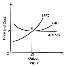
Under perfect competition, however, the demand curve (AR) is tangential to the long-run average cost curve (LAC) at its minimum point and conditions of full equilibrium are fulfilled: LMC = MR and AR (price) = Minimum LAC. This means that in the long-run the entry of new firms forces the existing firms to make the best use of their resources to produce at the lowest point of average total costs.
At point E in Figure 5 abnormal profits will be competed away because MR = LMC – AR = LAC at its minimum point E and OQ will be the most efficient output which the society will be enjoying. This is the ideal or optimum output which firms produce in the long-run.
Under monopolistic competition, the demand curve facing the individual firm is not horizontal, but it is downward sloping. A downward sloping demand curve cannot be tangent to the LAC curve at its minimum point. The conditions of equilibrium LMC = MR and AR (d) = Minimum LAC will not be fulfilled.
The firms will, therefore, be of less than the optimum size even when they are earning normal profits. No firm will have the incentive to produce the ideal output, since any effort to produce more than the equilibrium output would involve a higher long-run marginal cost than marginal revenue.
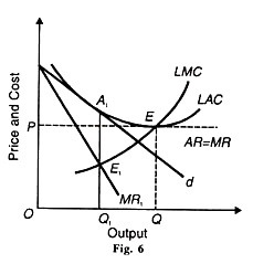
Thus each firm under monopolistic competition will be of less than the optimum size and work under excess capacity. This is illustrated in Figure 6 where the monopolistic competitive firm’s demand curve is d and MR1 is its corresponding marginal revenue curve. LAC and LMC are the long-run average cost and marginal cost curves.
The firm is in equilibrium at E1 where the LMC curve cuts the MR1 curve from below and OQ1 output is set at Q1A1 price. OQ1 is the equilibrium output but not the ideal output because d is tangent to the LAC curve at A1 to the left of the minimum point E1.
Any effort on the part of the firm to produce beyond OQ1 will mean losses as beyond the equilibrium point E, LMC > MR1 Thus the firm has negative excess capacity measured by QQ1 which it cannot utilise working under monopolistic competition.
A comparison of the equilibrium positions under monopolistic competition and perfect competition with the help of Figure 6 reveals that the output of a firm under monopolistic competition is smaller and the price of its product is higher than under perfect competition.
The monopolistic competitive output OQ is less than the perfectly competitive output OQ and the monopolistic competitive price Q1A1 is higher than the competitive equilibrium price QE. This is because of the existence of excess capacity under monopolistic competition.
Chamberlin’s Concept of Excess Capacity:
Prof. Chamberlin’s explanation of the theory of excess capacity is different from that of ideal output under perfect competition. Under perfect competition, each firm produces at the minimum point on its LAC curve and its horizontal demand curve is tangent to it at that point.
Its output is ideal and there is no excess capacity in the long-run. Since under monopolistic competition the demand curve of the firm is downward sloping due to product differentiation, the long-run equilibrium of the firm is to the left of the minimum point on the LAC curve.
According to Chamberlin, so long as there is freedom of entry and price competition in the product group under monopolistic competition, the tangency point between the firm’s demand curve and the LAC curve would lead to the “ideal output” and no excess capacity. This is because consumers want product differentiation and they are willing to accept increased production costs in return for choice and variety of products that are available under monopolistic competition. However, the difference between actual outputs and ideal output under non-price monopolistic competition creates excess capacity.
It’s Assumptions:
Chamberlin’s concept of excess capacity assumes that:
(i) The number of firms is large;
(ii) Each produces a similar product independently of the others;
(iii) It can charge a lower price and attract other’s customers and by raising its price will lose some of its customers;
(iv) Consumer’s preferences are fairly evenly distributed among the different varieties of products;
(v) No firm has an institutional monopoly over the product;
(vi) Firms are free to enter its field of production;
(vii) The long-run cost curves of all the firms are identical and are U-shaped.
Explanation:
Given these assumptions, excess capacity arises when there is no active price competition despite free entry of firms in a monopolistic competitive market.
Chamberlin gives the following reasons for such a situation:
(i) Firms may consider costs rather than demand in fixing prices,
(ii) They may aim at ordinary profits rather than maximum profits.
(iii) They may follow a policy of ‘live and let live’ and may not resort to price reduction,
(iv)They may have formal or tacit agreements, open price associations, trading association activities in building up esprit de corps and price maintenance,
(v) There may be the imposition of uniform prices on dealers by manufacturers,
(vi)Firms may resort to excessive differentiation of the product in an attempt to turn attention away from price cutting,
(vii) Business or professional ethics prevent firms from resorting to active price competition.
When there is no-price competition due to the prevalence of these factors, the curve dd is of no significance and the firms are only concerned with the group DD curve. Suppose the initial short-run equilibrium is at S where the firms are earning super-normal profits because the price OP corresponding to point S is above the LAC curve. With the entry of new firms in the group, super-normal profits will be competed away.
The new firms will divide the market among themselves and the group demand curve DD will be pushed to the left as D’D’ in Figure 7 where it becomes tangent to the LAC curve at point A. This point A is of stable equilibrium in the absence of price competition for all firms in the group and they are earning only normal profits. Each firm is producing and selling OQ output at QA (=OP) price.
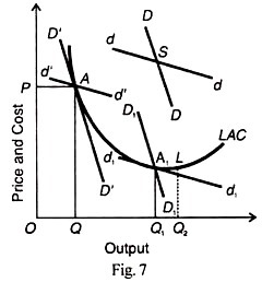
In Chamberlin’s analysis, OQ1 is the ‘ideal output’ without excess capacity, because each firm’s demand curve d[d] and the LAC curve are tangent at point A1 under price competition. But each firm in the group is producing OQ output in the absence of price competition. Thus OQ1 represents excess capacity due to competition under non-price monopolistic competition.
Chamberlin concludes that when over long periods under non-price competition prices do not tall and costs rise the two are equated by the development of excess productive capacity which does not possess automatic corrective.
Under monopolistic competition it may develop over long periods with impunity, prices always covering costs, and may, in fact become permanent and normal through a failure of price competition to function. The surplus or excess capacity is never abandoned and the result is high prices and wastes. They are the wastes of monopolistic competition.
Its Significance:
The concept of excess capacity is of much practical significance. Prof. Kaldor has characterised it as “intellectually striking”, ‘a highly ingenious’ and ‘revolutionary doctrine.’ It demonstrates an untraditional possibility that an increase in supply may lead to a rise in price.
The ‘wastes of competition’ which were hitherto a mystery have been unfolded. They pertain to monopolistic competition rather than to perfect competition, as was wrongly implied by the earlier economists.
It establishes the truth of the proposition that perfect competition and increasing returns are incompatible and proves that falling costs ultimately lead to monopoly or monopolistic competition. When monopolistic competition prevails, the number of firms will be large.
But each firm will be of a smaller size than under perfect competition. This entails a wasteful use of resources by bringing up firms with lower efficiency. Such firms use more manpower, equipment and raw materials than is necessary. This leads to excess or unutilized capacity.
Mostly excess capacity is due to fixed prices. But where price are not fixed, the entry of new competitors will raise elasticities of demand, lower prices and profits. If consumers’ inertia is present, prices will exceed costs and profits are not likely to fall. Thus excess capacity and superfluity of firms are bound to remain under monopolistic competition, as is the case in the present-day world.
Essay # 5. Selling Costs:
Selling costs are the expenses on advertisement, salesmanship, free sampling, free service, door-to-door canvassing, and so on. There is no selling problem under perfect competition where the product is homogeneous.
This is because the firm can sell at the ruling market price any quantity of its product. Therefore, there is no need for advertising. If, however, all firms want to sell more, competition among them will lead to price reduction until the new equilibrium price is reached. Each can sell as much as it wants to sell at this price.
Under monopoly also, selling costs are not required as there are no competitors. But the monopolist may sometimes advertise his product to acquaint the people about the use and price of his product so that they may continue to buy his product.
Under monopolistic competition where the product is differentiated, selling costs are essential to push up the sales. They are incurred to persuade a buyer to purchase one product in preference to another. Chamberlin defines them “as costs incurred in order to alter the position or shape of the demand curve for a product.”
He regards advertisement of all types as synonymous with selling costs. But in the present-day business nomenclature, the term selling costs is wider than advertising and it includes besides advertising, expenses on salesmen, allowances to sellers for window displays, free service, free sampling, premium coupons and gifts, etc.
Production Costs vs. Selling Costs:
Since each firm has to incur selling costs under monopolistic competition, its total costs include production costs and selling costs. Production costs include all expenses incurred in making a particular product, and transporting it to its destination for consumers.
They are the outlays on the services of all factor-services, land, labour, capital and organisation, engaged in the manufacture of the product and also include packaging, transport and service charges. Selling costs are costs incurred to change consumers’ preferences for a particular product.
They are intended to raise the demand for one product rather than another at any given price.
Prof. Chamberlin distinguishes between the two in these words:
“The former (production) costs create utilities in order that demand may be satisfied, the latter create and shift the demand curves them.” To be precise, “those which alter the demand curve for a product are selling costs and those which do not, are production costs”.
In other words, “those made to adapt the product to the demand are production costs and those made to adapt the demand to the product are selling costs.”
However, no clear-cut distinction can be made between production costs and selling costs. Is the cost of a cellophane wrapper, for instance, a production cost or a selling cost? In fact, “the two types of costs are interlaced throughout the price system, so that at no point such as at the competition or manufacture, can one be said to end the other to begin.”
But Prof. Chamberlin himself finds a way out by confining selling costs to only advertising expenses.
The Curve of Selling Costs and Its Influence on Production Costs:
The curve of selling costs is a tool of economic analysis forged by Prof. Chamberlain. It is a curve of average selling cost per unit of product. It is akin to the average cost curve and like the latter is U-shaped. Under the influence of the law of variable proportions, the curve of selling costs first falls, reaches a minimum point and then starts rising as shown in Figure 8.
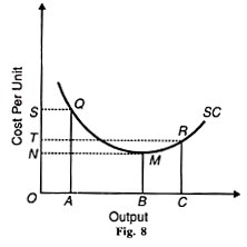
SC is the curve of selling costs. AQ is the average cost of selling OA units of the product, the total cost of selling it being OAQS. At the minimum point M of the SC curve, the cost per unit of selling OB units is BM which is less than any point in the QM portion of the SC curve. After this point, the average selling cost of ОС units is RC, the total cost of selling this quantity of the product being OCRT.
In fact per-unit selling cost and total selling costs increase beyond the minimum point M. According to Chamberlin, the shape of the curve and the exact point where it moves upward depends upon the nature of the product, its price, the nature of competing substitutes, the incomes of the buyers and their reluctance to change their tastes by the advertisement.
There is, however, a limit to the rising portion of the selling cost curve.
When the sales reach the saturation point, it ultimately becomes vertical. In the beginning, the application of successive doses of selling costs will raise the total sales more than proportionately so that average selling costs fall. This is due to two factors; firstly, consumers being attached to a particular brand of the product say, Brooke Bond Tea, are in the habit of buying it alone.
Advertisement in favour of another variety of the same product says Tata Tea, is meant to break their habit and dissolve the attachment of consumers to Brooke Bond Tea. One or two insertions a month in newspapers may make little impact on the consumers.
To convert the buyers to its brand, the manufacturer will have to incur larger selling outlays in the form of repetitive insertions of advertisement in newspapers, in commercial broadcasts, on the TV, in the form of samples, gifts or premium coupons.
Then only, sales will increase. Secondly, as larger outlays are incurred on sales promotion, internal economies of advertisement appear in the form of efficient salesmen, attractive advertisements and packing, etc. For instance, the larger the insertions and the size of advertisement, the lower the advertising rates per page. Thus, these two factors tend to lower average selling costs per unit of product up to a point.
Beyond this critical output M in our figure, average selling costs start rising again due to two forces. One, progressively increasing sales promotional expenses is to be incurred to induce regular consumers to continue to buy it.
Efforts to induce old customers to buy the same product require larger promotional expenses so that they are not only dissuaded from buying some other brand but also persuaded to buy more of the same product.
Two, larger selling outlays are required to attract new customers and those attached to other brands of the same product. They have to be convinced by repetitive advertisements in newspapers, through the radio, the cinema and television, of the superiority of this particular brand. Naturally such efforts require increased selling expenses.
As a consequence of these forces, average selling costs per unit of the product rise. We may conclude that two sets of forces operate in response to selling outlays on a product which tend to bring increasing returns up to a point, and beyond that, diminishing returns.
Proportional Selling Costs:
Average selling costs have the effect of raising the average total cost of production. If the average selling costs are proportional to the product sold, the curve of average total costs will lie at an equal distance above the average product cost curve.
For instance, when with a Signal toothpaste, a packet of five Erasmic blades is given free; the cost of five Erasmic blades incurred by the makers of the toothpaste represents proportional selling costs.
The product cost per unit of toothpaste and the selling cost per unit of a packet of blades added up from the total cost per unit of a tooth- paste-cum-five blade. The average production costs will rise by the cost of blades and will remain the same so long as the firm continues to sell in this proportion. This is illustrated in Figure 9 where APC represents the average production costs curve and AC the average costs curve.

The average costs are proportional throughout. They remain the same at all levels of output. At OQ output they are BA and even at OM level of output, they are the same as before DC (=BA), so is the average total cost MC (=QA). It should be noted that the corresponding MC curves of A PC and AC will also move in the same proportion (not shown in the figure).
We have assumed here that the producer continues to incur proportional selling costs which are unrealistic. In fact, a producer will resort to proportional selling costs only for a short while till his old stock is exhausted and in the process he also attracts new customers and induces regular users to buy more of it.
Fixed Selling Costs:
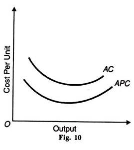
Selling costs are also of a fixed type, as in the case of screening a short-film in a cinema for a month or an insertion in the newspaper each Sunday. The average total cost per unit will at first be higher and as output increases it will fall and then, after a point, will start rising and the average total cost curve gradually becomes closer to the average production cost curve, as output increases further.
It implies that as sales increase, fixed selling costs are spread over a larger output and become less and less as shown in Figure 10, where APC represents the average production cost curve and AC the average total cost curve inclusive of selling costs.
The corresponding MC curves to APC and AC would be derived in the same manner and bear the same relation to their respective average cost curves. Added together they would give a combined MC curve (not shown in the figure).
Sometimes, certain tailoring and dry-cleaning concerns provide free home delivery service to their customers. But in such cases the effect of home delivery service is difficult to calculate on average and marginal costs.
Influence of Selling Costs on the Demand Curve:
The purpose of selling costs is to influence the demand curve for the product of a firm or group. A producer incurs selling costs in order to push up his sales. Therefore, all selling costs tend to shift an individual seller’s demand curve to the right.
The question of a demand curve shifting to the left is altogether ruled out in this analysis. When the demand curve for the product of a firm shifts to the right, it is the result either of inducing the same customers to buy more of the same product or new customers buying this product attracted by the advertisement.
The new demand curve may be more or less elastic throughout its length or parts of it may be more or less elastic than the old demand curve before incurring selling costs. If the buyers are convinced of the superiority of this product in contrast with other similar products, the new demand curve will be less elastic in the upper segments than the old demand curve.
The firm will be losing few customers as a result of rise in the price of its product.
If, on the other hand, the old and the new customers are attracted more to the product, but, at the same time, are not prepared to pay a very high price, the new demand curve will be highly elastic in its lower portion.
Besides, the buying habits of the old and new customers also influence the shape of the demand curve. If they are influenced more by price changes rather than the product variation, the new demand curve will be highly elastic.
On the contrary, if they are not influenced much by price changes, the new demand curve will be less elastic than the old curve. In the analysis that follows straight-line demand curves are taken for the sake of simplicity.
When the new demand curve is drawn parallel to the old, the elasticity of demand on the higher curves is lower at each price. It means that the consumers are convinced of the superiority of this product and are willing to pay a higher price.
Price-Output Determination under Selling Costs:
Under monopolistic competition, an individual firm has a variety of choices to sell a larger output. It may do so by lowering the price of the product; it may improve its quality; it may indulge in greater sales promotion efforts or it may resort to all the three methods simultaneously or combine the one with the other. We shall, however be concerned with only selling costs.
But even this problem is complicated because to depict each level of output at each price and the possible AR, MR, MC, and AC curves on a two-dimensional figure become complex. So for the sake of simplicity, the demand curve and the average total cost curve are taken along with the average production cost curve.
The following analysis discusses the influence of the selling costs on the price-output policy of the firm and the group.
Firm’s Equilibrium under Selling Costs:
This analysis assumes that when a firm incurs selling costs:
(1) Its demand curve shifts upward to the right;
(2) The average total cost curve lies above the average production cost curve; and
(3) The firm maximises its net profits.
Since MC and MR curves are not shown in the diagram, the formula for calculating net profits is: Net Profits = (Price x Output)-(Production Costs + Selling Costs), i.e., the difference between the new demand curve and the average total cost curve multiplied by the number of units of the product sold at that price.
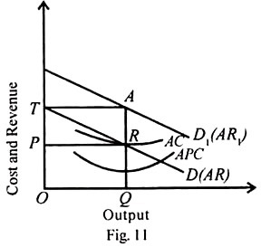
(1) Price Changes, Product and Selling Costs Remain Constant:
First we take the case of proportional selling costs with the assumption that only price change, sales remaining constant. The original demand curve is D (AR) and D1 (AR1) is the new demand curve. APC is the average production cost curve and AC is the average total cost curve, inclusive of selling costs.
The average total cost curve = average production costs + average selling costs. The firm maximises its output OQ at QA price and earns net profits measured by the area PRAT, as shown in Figure 11.
(2) Selling Costs Fixed, Price and Product Vary:
Suppose a firm spends Rs.1000 on advertising its product. Every time it spends this sum of money, the demand curve for its product shifts. In Figure 12, APC is the production cost curve and each time when Rs.1000 are spent on advertising, the average total cost curve becomes AC1 and AC2. D (AR) is the original demand curve before selling costs are incurred and D1 (AR1) and D2 (AR2) are the new demand curves.
The original equilibrium position is when OA output is sold at OP price. The firm earns TSRP super-normal profits.
Now, when selling costs are incurred in the first instance, the new equilibrium position brings T1S1R1P1 profits by selling OB output at OP1 price. Further expenditure of Rs.1000 on advertising increases profits to T2 S2 R2 P2, when ОС quantities of the product are sold at OP2 price.
The firm will, however, continue to spend Rs. 1000 on advertising its product each time so long as it adds more to total revenue than to total costs, till profits are maximised.
If the firm spends more on advertisement beyond this level, the addition to revenue will be less than costs. The firm will lose rather than gain by increasing selling costs. In Figure 12 the firm reaches the position of maximum profits when ОС product is sold at OP2 price and the firm earns T2S2R2P2 super-normal profits. Any further expenditure on advertisement will lead to diminution of profits.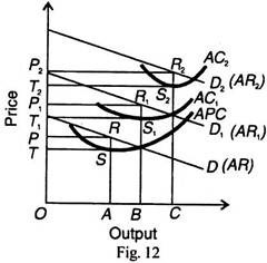
Essay # 6. Wastes of Monopolistic Competition:
From the point of view of economic efficiency or welfare as compared to perfect competition, monopolistic competition tends to reduce economic efficiency through a number of wastes such as unutilised or excess capacity, malallocation of resources, advertising, product differentiation, etc.
They are also called wastes of competition but it is more appropriate to characterise them as ‘wastes of monopolistic competition or of imperfect competition’. As pointed out by Professor Chamberlin “Many of the so-called wastes of competition are really wastes not of pure competition but of monopolistic competition”. Some of these are discussed below.
1. Competitive Advertisement:
One of the important wastes of monopolistic competition is the incurring of expenditure on competitive advertisement by firms. Excess advertisement adds to costs and prices. Expenditure on packing, colour, flavour, etc. and on media like TV, radio, cinema, newspapers, etc. create unnecessary product differentiation.
As a result, irrational preference for certain brands of products are created in the minds of consumers which tend to push the sales of one firm at the cost of others. Expenditure of competitive advertisement is also resorted to by all firms at least to keep their respective customers attached to their brand of the product. But all such expenditure is socially wasteful.
2. Product Differentiation:
Another waste of competition is the production of varieties of a product which each firm produces. This is done by creating artificial or imaginary product differentiation so as to distinguish the product of one seller from those of another. This is done by changing the colour, design, fragrance, packing, etc. of the same product by the same producer. For instance, The Brooke Bond Tea Company sells such brands of tea as Green Label, Red Label, Yellow Label, etc.
Thus each firm produces varied assortment of types and qualities for its own customers and often confusing them. Rather than producing only one type of product and charging uniform price, they charge different prices for each brand of the same product. Thus a large number of brands, styles, etc. confuses the consumer and adds to costs and prices, thereby making the products costly. This leads to wastage of resources and to loss of economic efficiency.
3. Expenditure on Cross Transportation:
The expenditure on cross transport is another waste of monopolistic competition. Each producer tries to sell his products in the far-off markets rather than in the markets near its place of manufacture. This involves huge transport costs and also expenses on advertisement and propaganda. Rather than save these expenses and reduce prices, firms under monopolistic competition prefer to incur expenses on transportation and advertisement. This is apparently wastage of resources.
4. Inefficient Firms:
Under monopolistic competition, there is a large number of inefficient firms. The price charged by each firm exceeds the long-run marginal cost because both the AR and MR curves are downward sloping under monopolistic competition. The firm’s equilibrium condition is Price=LAC>LMC=MR. Therefore, resources are under allocated to firms in the market and misallocated in the economy.
Under perfect competition all firms are of the most efficient size in the long-run because P=LAC=LMC=MR. Moreover, under monopolistic competition, an inefficient firm will have to lower its price in order of sell more and to expand. For this, it will have to lower its average costs per unit. But an inefficient firm may not be in a position to lower its average costs per unit and to lower its price.
Thus such firms may continue to exist on the strength of their customers but without attracting the customers of their rivals. There are a number of small retail shops in every town which depend upon the goodwill of their customers who due to ignorance or transport costs would not like to move to more efficient firms which sell the same product at a lower price. But the existence of such inefficient firms is a social waste.
5. Excess Capacity:
All firms under monopolistic competition possess excess capacity. Since the demand curve (AR) of a monopolistic competitive firm is downward sloping, its tangency point with the LAC curve will always occur to the left of its minimum point. Thus when the firm is in long-run equilibrium, it underutilizes its optimum scale plant. This leads to the existence of more firms in the industry than required.
All firms work under less than the optimum capacity, and all charge higher than the competitive price. The failure of the firms to produce less than the optimum output due to a downward sloping demand curve is a clear wastage of resources from the point of view of the community.
6. Unemployment:
As a corollary to the above, unutilized resources lead to unemployment when firms under monopolistic competition try to maintain the price of their product instead of maintaining production.
Conclusion:
From the above, it should not be inferred that monopolistic competition is sheer wasteful and reduces economic welfare. It has also its merits. For example, informative advertisement is useful for consumers and product differentiation provides the consumer a wider choice of products.