The Equilibrium of Money: An Overview

The Equilibrium of Money: An Overview!

Introduction:

We will examine the decisions involving the allocation of wealth among different Assets.

Thus, decision-making in this sector is called the money sector, because we concentrate on the allocation of wealth between money and all other assets — here we shall represent by bonds.

We make this particular subdivision of the wealth sector because money represents command over resources; each individual can exchange it for goods and services, even though the economy as a whole cannot.

Money does not refer to all wealth but to one type of wealth. Money is the stock of assets that can be readily used to make transactions.

The Functions of Money:

Money has three functions. It is a medium of exchange, an unit of account and a store of value.

As a medium of exchange, money is what we use to buy goods and services. ‘It is a legal tender for all debt’ is printed on the U.K. pounds. When we walk into stores, we are confident that the shopkeeper will accept our money in exchange of the goods they are selling. To understand this function of money, try to imagine an economy without it; a barter economy. In such a world, trade requires the double coincidence of wants. A barter economy permits only simple transactions.

As an unit of account, money provides the terms in which the prices are quoted and debts recorded.

As a store of value function of money, it is a way to transfer purchasing power from the present to the future. If I earn today £100, I can hold the money and spend it tomorrow, next week, or next month.

Of course, money is an imperfect store of value:

If prices are rising, the real value of money is falling. Even so people hold money because they can trade the money for goods and services at sometime in the future.

Types of Money:

Money that has no intrinsic value is called fiat money, since it is established as money by government decree. Although today fiat money is the norm in most economies, historically most societies used for money a commodity with intrinsic value. This type of money is called commodity money. Gold is the most widespread example of commodity money.

An economy in which gold used as money is called gold standard. Gold is a type of commodity money because it can be used for many other purposes apart from transactions. The gold standard was common during the late 19th century.

From Commodity Money to Fiat Money:

It is not surprising that some form of commodity money arises to facilitate exchange; people are willing to accept a commodity money because of its intrinsic value. The development of fiat money is more perplexing. What would make people begin to value something that is intrinsically useless?

To understand how it evolved from commodity money to fiat money, imagine an economy in which people carry around bags of gold. When purchase is made, the buyer measures out the appropriate amount of gold. If the seller is convinced about the weight and purity of gold, the buyer and seller make the exchange.

The government first intervenes to reduce transaction cost — time it takes to verify the purity and to measure the correct quantity of gold. To help reduce these costs, the government mints gold coins of known purity and weight. The coins are easier to use than gold bullion because their values are widely recognised.

The next step for the government is to issue gold certificate — pieces of paper that can be redeemed for a certain quantity of gold. These bills are just as valuable as the gold itself. In addition, because the bills are lighter than the gold, they are easier to use in transactions.

Eventually, these gold-backed government bills, instead of gold, became the monetary standard. Finally, the gold backing becomes unnecessary. As long as everyone continues to accept the bills in exchange, they will have value and serve as money. Thus, the system of commodity money evolves into a system of fiat money.

How Money Is Controlled:

The quantity of money available is called the money supply. In an economy that uses fiat money, the government controls the money supply. Just as the level of taxation and the level of government purchases are policy instruments of the government, so is the supply of money. The control of money supply, in all countries is delegated to an institution called the Central Bank. The control of money supply is called monetary policy.

The primary way in which the Central Bank controls the money supply is through open-market operations — the purchase and sale of government bonds. The purchase increases the quality of money supply, whereas, the sale decreases its supply.

How The Quantity Of Money Is Measured:

Let us examine how economists measure the quantity of money. Because money; is the stock of Assets used for transactions, the quantity of money is the quantity of those assets. The most obvious asset to include in the quantity of money is currency, the sum of fiat money — paper money and coins. Most day-to-day transactions use currency as the medium of exchange.

A second type of asset used for transactions is Current Account or Checking Accounts. If most sellers accept personal checks, assets in a Checking Account’ or Current Account are almost as convenient as currency. In both cases, the assets are in a form that is ready to facilitate a transaction. Thus, Current Account deposits are added to currency when measuring the quantity of money.

Once we admit the logic of including Current Account in the measured money stock, many other assets become candidates for inclusion. Funds in Savings Accounts, for example, can be easily transferred into Checking Accounts; these assets are almost as convenient for transactions.

Since it is unclear exactly which assets should be included in the money stock, various measures are available. Table 1 presents several measures of the money stock which are regarded as money especially in the U.K.

The Quantity Theory of Money:

Having defined what money is and examined how it is controlled and measured, we can now analyse how the quantity of money affects the economy. For this we need to see how the quantity of money is related-to other economic variables.

People hold money to buy goods and services. The more money they need for transactions, the more money they hold—thus, the quantity of money is closely related to number of transactions.

The link between transactions and money expressed in the following quantity equation:

MV = PT, where T represents the total number of transactions during some period of time, say, a year; P is the price of a typical transaction.

The product of the price of a transaction and the number of transactions, PT, equals the number of money exchanged in a year.

M is the quantity of money and V is called the transaction velocity of money and measures the rate at which money circulates in the economy. For example, suppose that 60 loaves of bread are sold in an economy in a given year at a price of £0.50 per loaf. Then T = 60 loaves per year, and P = £0.50 per loaf. PT = £0.50 x 60 = £30. Thus, the right-hand side of the quantity equation equals £30 per year, which is the money value of all transactions.

Suppose further that the quantity of money in the economy is £10. Then V = PT/M = 30/10 = 3 times per year. The quantity equation is an identity; the definitions of the four variables make it true. The equation is useful because it shows that if one of the variables changes, one or more of the others must also change to maintain the equality. For example, if the quantity of money increases and the velocity of money remains unchanged, then either the price or the number of transactions must rise.

From Transactions to Income:

Economists use a slightly different version of the quantity equation. The problem with the previous equation is that it is difficult to measure the number of transactions T. Thus, the number of transactions T is replaced by the total output of the economy Y. If Y denotes the amount of output and P is the price of one unit of output, then the money value of output is PY.

In other words, Y is real GDP; P is the GDP deflator, and PY nominal GDP. The quantity equation becomes MV = PY. Because Y is total income, V is called the income velocity of money. This version is the most common and is useful for economic analysis.

Money Demand Function and the Quantity Equation:

The demand for money is a demand for real balances. In other words, people hold money for its purchasing power, for the amount of goods they can buy with it. This amount is M/P and is called real money balances. People are not concerned with their nominal money holdings.

An individual is free from money illusion if a change in the level of prices, holding all real variables constant, leave the person’s real behaviour, including real money demand unchanged. By contrast, an individual whose real behaviour is affected by a change in the price level, all real variables remaining unchanged, is said to suffer from money illusion.

A money demand function is an equation that shows what determines the quantity of real money balances people wish to hold for transaction purposes. A money demand function is (M/P)^D= kY, where k is a constant. This equation states that the quantity of real balances demanded is proportional to real Y. Holding money makes it easier to make transactions. So higher Y leads to a great demand for money balances (M/P).

The quantity equation can be derived from this money demand function. To do so we add the condition that (M/P)^d must equal the (M/P) supply. Thus, (M/P)^d – (M/P) – kY.

Rearranging the terms we can write:

M (l/k) = PY, where V = l/k. We can write this as MV = PY.

Hence, when we use quantity equation, we assume that the supply of real money balances equals the demand which is proportional to income.

The quantity equation can be transformed into useful theory—the quantity theory of money — by making additional assumption that velocity is constant. This assumption of constant velocity provides a good approximation to reality. Let us see what this assumption implies about the effects of the money supply on the economy.

Once the assumption of constant velocity is accepted, the quantity equation can be seen as a theory of nominal GDP. The quantity equation says MV = PY, where V means fixed velocity. Therefore, a change in the quantity of money (M) must cause a proportional change in nominal GDP (PY). That is, the quantity of money determines the money value of the economy’s output.

The Demand for Money:

People hold money though it is not costless. Money, unlike other assets, does not yield an explicit rate of return. It is thus a relevant question to ask what money gives which makes individuals willing to pay the price to hold it. There are three motives for holding money – the transactions motives, the speculative motive, and the precautionary motive. The transactions motive arises from the function of money as a medium of exchange.

Most economic activity involves exchange and barter is an inconvenient and expensive way of making exchanges. Money is an asset which is generally acceptable as a medium of exchange and can be easily exchangeable for goods and other assets. One of the reasons for holding wealth in the form of money is that it allows us to make transactions without undergoing the costs and incon­veniences of converting some other assets into money.

For this particular motive, it seems reasonable that the two variables which would be important in determining how much money people want to hold are the volume of transactions, and the cost of holding wealth in the form of money. The first of these variables can be represented by real income (Y), because the higher is Y the greater will be the volume of transactions.

The cost of holding money is forgone interest rate, which shows what could be earned if wealth were held in the form of interest-bearing assets, rather than in the form of money. People decide how much money to hold on the basis of costs and benefits.

Transaction theories explain the money demand function which is known as the Baumol-Tobin model and it remains a leading theory of money demand today.

Keynesian analysis assumes that transactions demand for money is a function of income and it is not dependent on the level of income.

The Supply of Money:

Here we see that the banking system plays a key role in determining the money supply, and in most countries the only supplier of currency is some central authority, for example, the Issue Department of the Bank of England. We discuss various instruments that the Central Bank can use to alter the money supply.

We can thus treat the supply of currency as being exogenous, possibly affecting the economic system but not being affected by it, except so far as the central authority decides it wants to be affected. We defined the quantity of money as the amount of money held by the public, and we assumed that the Central Bank also controls the money supply by increasing or decreasing the quantity of money in circulation through open-market operations. Although this explanation is acceptable as a first approximation, it is not complete because it omits the role of the banking system in determining money supply.

Thus, the money supply is determined not only by the Central Bank, but also by the behaviour of households which hold money and of banks in which money is held. The money supply includes both currency in the hands of the public and the deposits of banks that households can use on demand for transactions.

That is, if M denotes the money supply, C currency, and D demand deposits, we can write:

Money Supply (M) = Currency (C) + Demand Deposits (D) To understand the money supply, we must understand the interaction between currency and demand deposits and how Central Bank influences these two components of the money supply.

100-Percent Reserve Banking:

Suppose that banks accept deposits but do not make loans. The only purpose of the banks is to provide a safe place for depositors to keep their money. The deposits that banks receive but do not lent out are called Reserve. In this simple economy, all deposits are held as Reserves – banks accept deposits, place the money in reserve until the depositor makes a withdrawal. This system is called 100-Percent Reserve Banking.

A Balance Sheet of a bank under 100-Percent Reserve Banking looks like Fig. 1. A bank’s Balance Sheet shows its assets and liabilities. Under this system, banks hold deposits as reserves. If the bank holds 100% of deposits in reserve, the banking system does not affect the supply of money.

Fractional-Reserve Banking:

In most countries, the banking system operates on a partial reserve basis which means banks use some of their deposits to give loans. The banks keep some fraction of their deposits on hand so that reserves are available whenever depositors want to make withdrawals. The banks have a legal requirement to hold some fraction of their deposits in the form of some particular assets, known as Reserve Assets. This system is known as Fractional-Reserve Banking.

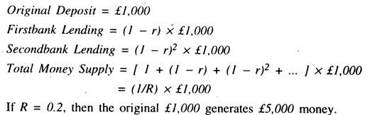
Fig. 2 shows the Balance Sheet of Fractional-Reserve Banking System. This Balance Sheet shows the maximum amount of deposits that the banks can create depends on reserve-deposit ratio — the fraction of deposits kept in reserve. We assume that the banks are required to keep 20% of their deposits as reserve ratio. First-bank keeps £200 of the £1,000 in deposits in reserve and lends out the remaining £800.

Thus, we can see that First-bank increases the supply of money by £800 when it makes this loan. Before the loan is made, the money supply is £1,000. After the loan is made, the money supply is £1,800, the depositor still has a demand deposit of £1,000, but now the borrower holds £800 in currency. Thus, under a fractional-reserve system, banks create money.

The creation of money does not stop with First-bank. If the borrower deposits the £800 in another bank, the process of money creation continues. Fig. 2(b) shows the Balance Sheet of Second-bank. Second-bank receives the £800 in deposits, keeps 20% or £160, in reserve, and then lends out £640, and so on, with each deposit and loan, more money is created.

Although this process of money circulation can continue, it does not create an infinite amount of money.

Let r denotes the reserve-deposit ratio, then the amount of money that the original £1,000 creates is:

The banking system’s ability to create money is the primary difference between banks and other financial institutions. Financial markets have the important function of transferring the economy’s resources from those house­holds that wish to save some of their income for the future of those households and firms that wish to borrow to buy investment goods to be used in future production. This process is called financial intermediation.

Many institutions in the economy act as financial intermediaries; the most important examples are the stock market, the bond market, and the banking system. Yet, of these institutions, only banks have the legal authority to create assets that are of the money supply, such as Current Accounts.

Thus, banks are the only financial institutions that directly influences money supply. It may also be noted that although the system of fractional-reserve banking creates money or liquidity, it does not create wealth.

A Model of the Money Supply:

We have seen how banks create money. Here we present a model of the money supply under fractional-reserve banking.

The model has three exogenous variables:

1) The monetary base B is the total amount of money held by the public as currency C and by the banks as Reserves R. It is directly controlled by the Central Bank.

2) The reserve-deposit ratio r is the fraction of deposits that banks hold in reserve. It is determined by the laws regulating banks.

3) The currency-deposit ratio C_r expresses the preferences of the public about how much money to hold in the form of demand deposits D and how much to hold in the form of currency C.

The model shows how the money supply depends on the monetary base, the reserve-deposit ratio, and the currency- deposit ratio. It allows us to examine how the policy of the monetary authority and the choices of banks and households influence the money supply.

We begin with the definitions of money supply and the monetary base:

M = C + D; B = C+ R

The first equation states that the money supply is the sum of currency and demand deposits. The second equation states that the monetary base is the sum of currency and bank reserves.

M/B = C + D/C + R.

Then divide the numerator and denominator by D, M/B = C/D + 1/ C/D + R/D.

We already know that C/D is the currency-deposit ratio C_r, and the R/D is the reserve-deposit ratio r. Substituting these and bringing B from the left to the right side of the equation, we get M = Cr + 1/Cr + r x B. This equation shows how the money supply depends on three exogenous variables.

Thus, the money supply is proportional to the monetary base. The factor of proportionality, (C_r + 1)/ (C_r + r) = m and is called the money multiplier.

We can write:

M = m x B.

Each pound of the monetary base produces m pounds of money. Because the monetary base has a multiplier effect on the money supply, the monetary base is sometimes called high-powered money. For example, in the US economy the monetary base is $300 billion, the reserve-deposit ratio r is 0.1 and the currency-deposit ratio, C_r, is 0.4. In this case, the money multiplier is m = 0.4 + 1/ 0.4 + 0.1 = 2.8 and the money supply is M = 2.8 x 300 = 840.

Each dollar of the monetary base generates 2.8 dollars of money, so that the total money supply is $840 billion.

We can now see how changes in three exogenous variables — B, r, and C_r — causes money supply to change:

1) The money supply is proportional to the monetary base. Thus, an increase in the monetary base increases the money supply by the same percentage.

2) The lower the reserve-deposit ratio, the more money loans banks can make and more money they can create. Thus, a decrease in the reserve-deposit ratio raises the money multiplier and the money supply.

3) The lower the currency-deposit ratio, the more money banks can create. Thus, a decrease in the currency-deposit ratio raises the money multiplier and the money supply.

The Three Instruments of Monetary Policy:

The monetary authority controls the money supply directly and/or indirectly by altering either the monetary base or the reserve-deposit ratio. To do this, the monetary authority has at its disposal three main instruments of monetary policy – open-market operations, reserve requirements and the discount rate.

Open-market Operations are the purchases or sales of government bonds by the Central Bank/monetary authority. When it buys bonds from the public, the money it pays for bonds increases the monetary base and thereby increases money supply. When it sells bonds to the public, the money it receives reduces the monetary base and thus decreases the money supply. Open-market operations are the most-often used policy instrument of the Central Bank.

Reserve Requirements are Central Bank regulations that impose on banks a minimum reserve-deposit ratio. An increase in reserve requirement raises the reserve-deposit ratio and thus lowers the money multiplier and the money supply. This is the least-frequently used instrument.

The discount rate is the interest rate that the Central Bank (BOE) charges when it makes loans to banks. Banks borrow from the Central Bank (CB) when they find themselves with too few reserves to meet reserve requirements. The lower the discount rate, the cheaper are borrowed reserves and the more banks borrow at the CB’s discount window. Hence, a reduction in the discount rate raises the monetary base and the money supply.

Although these instruments give the CB substantial power to influence the money supply, the CB cannot control money supply perfectly. Bank discretion in conducting business can cause the money supply to change in. ways the CB did not anticipate.

Money Market Equilibrium:

If investment is assumed to be a function of the rate of interest then we need to know the rate of interest to determine the equilibrium level of income. From the equality of saving and investment we can derive the equilibrium income, provided we know the interest rate. For this reason, we consider the determination of the interest rate in the Keynesian theory which is also known as liquidity preference theory.

According to Keynes, the interest rate is a monetary phenomenon. It depends on the supply of and the demand for money. Money is the most liquid asset. Liquidity is an important attribute of an asset. The more quickly an asset can be converted into cash without incurring any loss, the more liquid the asset is. Obviously money is the most liquid asset. The interest is the price paid for lending money or for partying the liquidity. Thus, the price of money or the rate of interest is determined by the equality of demand and supply of money.

The demand for money depends on three factors which Keynes called the ‘motives’ or ‘reasons’ for holding money.

These motives are:

1) The Transaction Motive.

2) The Precautionary Motive and

3) The Speculative Motive.

Let us now discuss these motives in more details.

1) The Transaction Motive:

The transaction motive arises from the function of money as a medium of exchange. An individual earns income after an interval of time, say a week, or a month, etc. During any two income- receiving periods, the individual will have to make transactions. In other words, the payments and receipts are not synchronised.

While the payments are made throughout the period, the income is received after a period of time. To carry out transaction during the period of time, an individual must hold a part of his income in the form of cash. Thus, the demand for money comes from its functions. Money acts as a means of payments or medium of exchange.

It also acts as a form of asset. Money balances kept by the people may be divided into two parts — active balance and idle balance. Active balance is held for the function of money as a means of payment, and idle money is held for its function as a form of asset.

Active balance is also called ‘transaction’ and ‘precautionary’ balances. In short, we call it transaction balance (M_t) which is assumed to be proportional to income.

So, the transaction balance of the economy will depend on the national income of the economy and can be written as:

M_t = kY….. (1), such that dM_t/dY > 0, where k is a positive constant.

Economists like Baumol, Tobin and others hold the view that the transaction balance of the economy depends not only on the level of income, but also on the rate of interest. If the rate of interest is higher, people will economise the use of cash, thereby reducing the average transaction balance of the economy.

2) Precautionary Motive:

Precautionary motive for holding cash arises, from the desire of the individual to hold some cash for meeting unforeseen events like, sickness, accident etc. To meet uncertain future obligations each individual will hold a part of his income in the form of money. Such cash balances are known as precautionary balances.

The difference between transaction demand and precautionary demand is that in the former case no uncertainty is involved. People hold money because payments and receipts are separated. But uncertainty is the source of precautionary demand.

People hold precau­tionary balances to meet uncertain circumstances. It also depends on the level of income. Thus, the precautionary balance- is a function of national income (Y), i.e., M_p = M_p(Y), such that dM_p/DY > 0, where M_p is the amount of precautionary balance and Y is income.

3) Speculative Motive:

It is the speculative motive for holding cash that makes the Keynesian theory of demand for money different from classical theory. Keynes considered the asset demand for money as idle balances. Keynes also assumed that there are two ways in which wealth can be held – money and bonds. If an individual holds money, he gets no interest income; on the other hand, if he holds bonds instead, he can get interest income. He can also make capital gains or losses by selling bonds at some future date.

Now the question is why should people hold money instead of bonds? The answer is that if he holds bonds he gets interest income. But he can also make capital gain or loss. Now if the sum of interest income and capital gain (loss) is positive, he will hold bonds. However, if the sum of interest income and capital loss is negative, he will hold only cash. Such idle balances which an individual holds rather than bonds is known as speculative balance or speculative demand for money.

Whether an individual holds money or bond depends on his expectations. Expectations are formed on the basis of his experience. If the current rate of interest is normal, people will expect it to prevail in the future. If the current rate is lower than the normal rate, the rate of interest will be expected to rise in the future and bond prices will fall.

On the other hand, if the current rate is lower than the normal, the rate of interest will fall in the future and bond prices will rise. However, expectations differ among individuals. The higher the current rate of interest above the normal rate, the greater is the percentage of people expecting the current rate to fall and vice versa. As the divergence between the current rate and the normal rate rises the percentage of people expecting the current rate to rise or fall also increases.

There are three assumptions regarding this function:

a) There is a maximum rate of interest (r_max) at which speculative demand for money is zero,

b) There is a minimum rate of interest (r_min) at which speculative demand is infinity — (r_min) is called the floor rate below which the rate of interest cannot fall), and

(c) Between these two extreme rates, the speculative demand for money is inversely related with the interest rate.

Thus, we can write the speculative demand for money as:

M_s = L(r)…….. (2)

where L’ (r) = ∞ for r = r_min,

L'(r) = 0 for r = r_max and L’(r) < 0 for r_min < r < r _max.

In Fig. 5.9, we draw the graph of equation (1) by measuring income horizontally and the transaction demand for money vertically. In Fig. 5.10, we plot the graph of equation (2) by measuring speculative demand for money horizontally and the rate of interest vertically. The total demand for money (M_d) is the sum of the transaction balance and the speculative balance.

Thus, the demand for money can be written as:

M_d = M_t + M_s = kY + L(r)…….. (3)

In its general form, the function can be written as:

M_d = L (Y, r)

where LY = k > 0,

and L_r obeys the same restrictions as those on L'(r).

Total demand for money will depend on the demand for active balances and on the demand for idle balances. Demand for active balances (M_t) is a function of the level of income while the demand for idle balances (M_s) is a function of the rate of interest. Total demand for money (M_d), is thus the sum of M_t and M_s; i.e., M_d = M_t + M_s = kY + L₂(r) = L (Y,r) …… (4)

Thus, the total demand for money (M_d) is a function of both the level of income and the rate of interest. This is known as the demand function of money or the liquidity preference function.

This function is such that ∂L/∂y > 0, ∂L/∂r < 0. This means that if the level of income remains the same, the demand for money varies with the rate of interest, or, if the rate of interest remains the same, the demand for money varies directly with the level of income.

The money market is in equilibrium, when the demand for money is equal to the given supply of money. When the demand for money exceeds the supply of money, some people will find that their demand for money is not satisfied. They-will sell bonds to acquire money. As a result, bond prices will fall and hence interest rate will rise.

Alternatively, when the supply of money is greater than demand, some people will hold too much money. They will try to get rid of excess money by buying bonds. As a consequence, bond prices will rise and thus interest rate will fall. Thus, to have equilibrium in the money market, the demand for money must equal its supply.

M_s = kY + L(r) = L (Y, r) …………. (5), where M_s is the institutionally given quantity of money supply in the economy.

In the Keynesian theory, it is assumed that the supply of money is given by the monetary authority. Total supply of money is independent of the rate of interest. The supply schedule can be represented by a vertical straight line.

Determination of the Equilibrium Rate of Interest:

The equilibrium rate of interest is determined by the supply and demand for money. Now we plot the demand and supply schedules in Fig. 5.11. The level of income is constant at Y₀ and the money demand function is CE and the supply of money is constant at OM₀ and the money supply curve is MM₀. The supply curve intersect the demand curve at A where the rate of interest is Or₀. Or₀ is the equilibrium rate.

At a higher rate of interest Or₁, the supply of money exceeds the demand for money. This excess supply of money at Or₁ is CD which pushes the interest rate towards Or₀. On the other hand, if the interest is Or₂, there will be an excess demand for money. The excess demand in the money market will push the interest rate towards Or₀.

This adjustment process can be expressed in terms of the follow­ing equation:

dr/dt =f(M_d – M_s), such that dr/dt > or = or < 0, according as (M_d – M_s) > or = or < 0,

where M_d is the demand for money and M_s is the supply of money.

In other words, it means that the rate of interest will decrease when there is excess supply of money, it will increase when there is an excess demand for money and will remain constant when there is no excess demand or supply (M_d = M_s).

Now let us consider the effect of an increase in the supply of money and its effect on the equilibrium rate of interest. As the supply of money increases, the money supply schedule shifts to the right. Suppose the supply of money increases from M₀ to M₁. The new equilibrium interest rate is Or₂ < Or₀.

Thus, when the money supply increases, the equilibrium rate of interest decreases. The reason is that since the level of income remains unchanged, the demand for active balance will also remain constant. The additional supply of money can be absorbed if the demand for idle balances (L) increases. Now L will increase only when the interest rate falls.

In other words, the additional supply of money will be diverted in the bond market thereby raising the demand and prices of bonds. This will mean a fall in the rate of interest. Thus, the supply of money reduces the equilibrium rate of interest.

Liquidity Trap:

If, however, the supply of money schedule intersects the demand schedule at the latter’s horizontal part, a further increase in money supply will not reduce the market rate of interest. In this situation, everyone will prefer cash to bonds and hence the additional supply of money will not increase bond prices and the rate of interest will not fall. In this situation, monetary policy will be ineffective.

For example, during a period of deep depression, when the rate of interest is very low and the liquidity preference schedule is completely interest-elastic, any increase in money supply will have no effect on the interest rate, income and employment. In this situation, monetary policy is said to be trapped and that is the reason why horizontal part of the money demand schedule is known as the liquidity trap. It sets a floor below which the interest rate cannot fall.

Criticism of the Keynesian Theory of Interest Rate:

Keynesian theory of interest rate determination has been criticised on the following counts:

First, in the Keynesian theory, the rate of interest cannot be determined unless the level of income is known. For one level of income, we shall get one equilibrium interest rate. If the level of income changes, the equilibrium interest rate also changes. Equilibrium rate of interest is, therefore, indeterminate in the Keynesian theory of interest rate determination.

In the money market, we have the following three equations and four unknowns:

r, Y, M, L.

1) M_d = M_t + M_s = kY + L(r)………………………. Money Demand Function

2) M = M₀……………………………………………… Money Supply Function

3) M_d = M………………………………………….. Equilibrium Condition

The system is indeterminate. The equilibrium condition can be written as:

kY + L(r) = M₀, where we get one equation and two unknowns r, Y.

Thus, we get different combinations of Y and r for which the above equation is satisfied. The locus of all combinations of r and Y gives us the LM curve. The LM curve gives us the money market equilibrium.

Secondly, Keynes ignores the influence of the real factors, such as, saving and investment in determining interest rate as he assumes it to be a monetary phenomenon. This seems unrealistic.

Thirdly, the Keynesian theory is a short-run theory. Only in the short run, an increase in the supply of money leads to a decrease in interest rate. However, if the supply of money generates inflationary expectations, then increase in the supply of money tends to raise rather than lower the interest rate.

Fourthly, in the Keynesian theory, an individual can hold either bonds or money but not both. But in the real world, individuals hold both. The Keynesian theory cannot explain this phenomenon.

Derivation of LM Curve:

In the money market, we get one money supply and money demand function and one equilibrium condition.

The money demand function is written as:

M_d = M_t + M_s = kY + L(r) , where M_d is the total demand for money, kY is the demand for active balances or transaction balances and L is the demand for passive balances or speculative balances.

The demand for active balances (M_t) depends on the level of income, while the idle balances (M_s) depends on the interest rate.

M_t is the constant fraction of money national income:

M_t = kPY , where Y is the real national income, P is the price level and k is the fraction of income people want to hold in the form of cash.

The M_S or L(r) is normally a downward-sloping function with two exceptions. There is a very high rate of interest at which M_s is zero and a low rate of interest at which M_s is infinitely interest-elastic. We also assume that the price level is constant at P₀ and M_t is an increasing function of income.

Hence the equilibrium condition in the money market can be written as:

M₀ = kP₀Y + L(r). This is a single equation with two unknowns r and Y. From this equation, we can get different combinations of r and Y for which demand for money is equal to the supply of money.

The locus of all such combinations gives us the LM curve as given in Fig. 5.12. From the given level of income, we know how much money will be kept for transaction balances (M_t = kP₀Y). Then the rest of the money supply, M – M_t, is available for speculative balances [M_s = L(r)] to determine the rate of interest which gives equilibrium in the money market.

Thus, corresponding to each level F, there is a rate of interest (r) which produces equilibrium in the money market. With a given quantity of money, we get a relation between Y and r which gives us the LM curve. The relationship is this — a rise in Y leads to an increase in the money required in the transaction balance, and thus, money available for speculative balance (M_s) is reduced; to get money released for transaction balance the rate of interest has to be increased. Then, a rise in Y leads to an increase in the rate of interest at which the money market is in equilibrium.

If the entire money supply is absorbed for transaction purposes, no money can be released from the speculative balance which has come down to zero. With a given quantity of money, income has a maximum limit above which it cannot rise. At this Y, the rate of interest would be maximum, Y_max, at which speculative demand is zero.

Conversely, a fall in income will reduce the transaction demand for money, and thus, money available for speculation will increase and the rate of interest will be reduced. If the rate of interest has already reached the floor, it cannot fall further. Then the extra money will be absorbed in the speculative balance without a further fall in interest rate.

Then, we have three phases of the LM curve:

A vertical phase where the speculative demand for money is interest-inelastic and the income has reached its highest attainable level and the rate of interest is r_max; a horizontal phase where speculative demand for money is interest-elastic for low levels of income where the interest rate stays at the floor level, Y_min; and, a positively sloped phase in between the two extremes.

A method of deriving the LM curve is given in Fig. 5.12. In the first quadrant, we can find the LM curve which shows the relationship between Y and r. In the second quadrant, we derive the speculative function, taking M as the origin. Any point on OM divides the total money between speculative balance (M_s) and the transaction balance (M_t).

The 45° line is drawn in the fourth quadrant to equate Y measured in two axes. In the third quadrant, we have plotted the M_t curve which is a straight line through the origin. Now we start from the interest rate r₁. At this rate of interest the demand for idle balances is MA and the money available for active balances is OA.

From quadrant three, we know that OA amount of active balance will be able to support Y₁ amount of income. Thus, we can say that when the interest rate is r₁ and the level of income Y₁, the money market is in equilibrium (i.e., the total demand for money is equal to the total supply of money). (Y₁, r₁) is a point on the LM curve and this point is shown in the first quadrant. Now, we consider a lower interest rate r₂ where M_s is MB and M_t is OB. At M_t of OB. income is equal to Y₂. Thus, we get another point (r₂, Y₂) on LM. Other points on the LM curve can be obtained in the same way.

It can be noted that as r increases, Y also increases; thus, we can say that LM curve is upward rising. Now if we take the interest rate of r₃, the income level is Y₃. At this rate of interest idle balance, M_s, is at horizontal part and the rate of interest has reached the floor level, so it cannot fall further. Whatever may be the level of income below Y₃, money demand will be equal to money supply at this rate of interest. The LM curve will thus be horizontal at the rate of interest r₃ and income Y₃.

Similarly, at the rate of interest r₄, the speculative demand (M_s) for money would be zero and Y₄ would be the corresponding level of income. At all rates of interest above r₄, Ms is equal to zero and the level of income will remain constant at Y₄. Thus, when the level of income has reached Y₄, the LM curve becomes vertical. The LM curve will have three parts—the horizontal part, the upward rising part and the vertical part.

These three parts correspond to the three positions of the M_s curve. When the M_s curve is horizontal, the LM curve is horizontal too. When the M_s curve is vertical, the LM curve is also vertical and when M_s curve is downward sloping, the LM curve is upward rising.

We made two assumptions when deriving the LM curve. One such assumption is that money supply is constant and the other assumption is that price level is constant as well. When any of these assumptions changes, the LM curve also will change its position. It will shift either to the left or to the right.

These three parts of the LM curve may be regarded as three ranges. The vertical part of the LM curve is known as classical range which is associated with the classical theory of money where money has no speculative role. The horizontal part of the LM curve is known as Keynesian range where the speculative demand for money is infinitely interest-elastic.

This situation can prevail only in deep depression. The upward sloping part of the LM curve is known as intermediate range. In this region, the speculative demand is neither zero nor infinitely interest-elastic.

The Slope of the LM Curve:

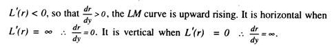
The equation of the LM curve is given by M_D = kP₀Y + L( r). Differentiating both sides with respect to Y we get,

Shift of the LM Curve:

If the real quantity of money is increased (reduced), the LM curve will shift to the right (left). This is shown in Fig. 5.13. In Fig. 5.13(b), we draw the demand for real money balances for a given level of income Y₁. With the initial money supply, M/P, the equilibrium is at point E₁, with interest rate at r₁. The corresponding point on the LM curve is E₁.

Now the real money supply increases from (M/P) to (M/P)’, which is represented by a rightward shift of the money supply schedule. To restore equilibrium in the money market at income level Y₁, the interest rate has to decline to r₂.

The new equilibrium is at E₂. This shows that in Fig. 5.13(a), the LM curve has shifted to LM’. At Y₁, the equilibrium interest rate has to be lowered to induce people to hold more money. Alternatively, income has to be increased to raise the transaction demand for money and thus to absorb the real money supply. Similarly, if the real money supply is reduced, the LM curve will shift to the left.