Properties of Isoquants | Production | Economics

The production function shows the relationship between the out­put of a good and the inputs (factors of production) required to make that good.

It usually takes the following general form:

Q = f (K, L, t, etc.)

Where Q is output, K is capital input, L is labour input, t is ‘technology or the art of production’ and the term ‘etc.’ indicates that other inputs may also be relevant (such as land, or raw materials). The production function shows how output changes are related to changes in inputs or factors of produc­tion. It is also an efficiency relation showing the maximum amount of output that can be obtained from a fixed amount of resources.

Production functions may take a variety of forms. Economists often work with homogeneous production functions. One example of such function is the famous Cobb-Douglas production function.

Production Isoquants:

The long-run production function involving the usage of two factors (say, capital and labour) is represented by isoquants or equal product curves (or production indifference curves).

Definition:

An isoquant is a curve or locus of points showing all possible combinations of inputs physically capable of producing a certain fixed level of output. An isoquant which lies above another shows a higher level of output.

Fig. 1 shows two typical isoquants — capital use is measured on the vertical axis and labour use on the horizontal. Isoquant Q₁ shows the locus of combinations of capital and labour yielding 100 units of output. The producer can produce 100 units of out­put by using 10 units of capital and 75 of labour or 50 units of capital and 15 of labour, or by using any other combina­tion of inputs on Q₁ = 100. Similarly, isoquant Q₂ shows the various combi­nations of capital and labour that can produce 200 units of output.

We can draw any number of iso­quants in Fig. 1 because there are an infinite number of possible production levels between 100 and 200 units (as also below 100 units or above 200 units).

Properties:

Isoquants have four important properties.

These are the following:

1. Firstly, an isoquant which lies above and to the right of another shows a higher level of output. So, any point on a higher isoquant is always better than any point on a lower isoquant.

2. Secondly, isoquants cannot meet or intersect one another. If they did, then one combination of K and L would yield two different levels of output. The producer’s technology is inconsistent. We rule out such events.

3. Thirdly, as shown in Fig. 1, isoquants slope downward over the relevant range of production. This negative slope indicates that, if the producer decreases the amount of capital employed, more labour must be added in order to keep the rate of output constant. Or, if labour use is decreased, capital use must be increased to keep output constant. Thus, the two inputs can be substituted for one another to maintain a constant level of output.

The marginal rate of technical substitution (MRTS):

The rate at which one input can be substituted for another along an isoquant is called the marginal rate of technical substitution (MRTS), defined as:

MRTS_{L for K} = – ∆K/∆L

where K is capital, L is labour and ∆ denotes any change. The minus sign is added in order to make MRTS a positive number, since ∆K/∆L, the slope of the isoquant, is negative.

For any movement along an isoquant, the MRTS equals the ratio of the marginal products of the two inputs.

To prove this, suppose the use of L increases by 3 units and K by 5. If, in this stage, the MP_L is 4 units of Q per unit of L and that of K is 2 units of Q per unit of K, the resulting change in output (Q) is:

∆Q = (4 x 3) + (2 x 5) = 22

This means that when L and K are allowed to vary slightly, the change in Q resulting from the change in the two inputs is the marginal product of L times the amount of change in L plus the marginal product of K times its change.

As a general rule:

∆Q = MP_L. ∆L + MP_K. ∆K.

Along an isoquant, Q is constant; therefore ∆Q equals zero. Setting ∆Q in the above equation equal to zero and solving for the slope of the isoquant, ∆K/∆L, we have:

∆K/∆L = MP_L/MP_K = MRTS_{L for K}

Since along an isoquant K and L must vary inversely, ∆K/∆L is negative.

4. Fourthly, over the relevant stage, the MRTS diminishes. This means that isoquants are convex to the origin. This point is illustrated in Fig. 1. If capital is decreased by 10 units, from 50 to 40, labour must be increased by only 5 units, from 15 to 20, in order to keep the level of output at 100 units. If capital is decreased by 10 units, from 20 to 10, labour must be increased by 35 units, from 40 to 75, to keep output at 100 units.

Optimal Combination of Resources:

A rational producer has the goal of either maximising output given a fixed budget (say, Rs. 300 per day) or minimising cost given a required output to produce (say, 150 units). Each goal is a problem of constrained optimisation.

Our task here is to determine the specific combinations of inputs a firm should select when it is constrained. Here we will observe that a firm attains the highest possible level of output for any given level of cost or the lowest possible cost for producing any level of output when the MRTS for any two inputs equals the ratio of their prices.

Input Prices and Isocost Lines:

The total cost, C, of using any value of K and L is C = r k + w L, the sum of the cost of K units of capital at a price of r per unit and of L units of labour at price of w per unit.

Suppose, capital costs Rs. 30 per unit (r = Rs 30) and labour receives a wage of Rs. 15 per day (w = Rs. 15). If only capital is used we have: C = r K + 0 and the maximum amount of capital that can be purchased is K = C/r = Rs. 300/Rs. 30 = 10 units. Similarly, if only labour is hired, we have: C = 0 + w L and the maximum number of workers that can be hired (per day) is L = C/w = Rs. 300/Rs. 15 = 20. We can also think of various other combinations of capital and labour that can be purchased (hired) with the same budget.

The budget equation is illustrated in Fig. 2. The line AB is called the isocost line or the line of equal cost. It is indeed the producer’s budget line.

Definition and Scope:

The isocost line is a locus of points showing alternative combinations of K and L that can be purchased with a fixed amount of money at prevailing market prices.

Its slope is:

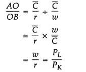
This is called the factor price ratio or the actual rate of factor substitution. Here, w is the price of labour (P_L) and r is the price of capital (P_K).

Output Maximisation subject to Cost Constraint:

A rational producer, whose ob­jective is output maximisation subject to cost constraint, will always try to reach the highest attainable isoquant permitted by the isocost line. This point is illustrated in Fig. 3. Here, the producer reaches Q₂ with his isocost line AB and produces 150 units of output at a cost of Rs 300. So, cost per unit is Rs. 2. Can total cost be reduced further?

No. If, through mistake or miscalculation, the producer moves to point F or G along the same isoquant, his total cost (outlay) will remain the same, but his output will fall to 100 units. So, his cost per unit will rise to 150 units. Thus, only point E can be an op­timal point. And the com­bination of K and L corresponding to the point (viz., K₁ and L₁) is called the least-cost com­bination. So, a rational producer maximises out­put by choosing the least- cost combination of inputs, the prices of which are taken as given (i.e., de­termined by market forces).

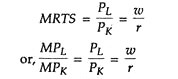
At point E the slope of the isoquant or MRTS is equal to the slope of the isocost line:

Production of a Fixed Output at the Lowest Cost:

Suppose, now, that the objective of the producer is to produce exactly 150 units of output, neither more nor less. This goal can also be achieved by choosing the least cost combination of inputs or by fulfilling the above condition. In Fig. 4 the only isoquant indicating an output of 150 units just touches the isocost line A₂B₂ at point E.

This meant that the minimum cost of producing a given output of 150 units is Rs. 2. If the producer moves to the right or left of point E along the same isoquant, cost will rise. Thus, E is the optimum point, indicating least cost combination of inputs. For ex­ample, at point on output is 30 units but total cost is Rs. 100 which means that cost per unit is Rs. 3.

Conclusion:

Thus, the two alternative strategies illus­trated here give the same results. In Order to maximise output subject to a given cost or to minimise cost subject to a given output, the producer must employ inputs in such amounts as to equate the marginal rate of technical substitution and the factor price ratio.