Isoquants (IQ) of a Firm: Assumptions, Properties and Types

In this article we will discuss about:- 1. Assumption of Isoquants and the Isoquant Map 2. Characteristics (Properties) of IQs 3. Types.

Assumption of Isoquants and the Isoquant Map:

For the sake of simplicity, we shall assume that the firm uses only two variable inputs, X and Y, and produces only one output Q. The production function of the firm, let us suppose, is

Let us suppose, q̅ = f(x, y) = xy (8.23)

Let us also suppose, q̅ = 100 units

Here from (8.23), we obtain that the firm’s output will be q = 100 units from any one of the input combinations: A (x = 5, y = 20), B (x = 10, y = 10), C (x = 20, y = 5), etc. If x and y are continuous variables, then we would get an infinitely large number of combinations like A, B, C,…. These combinations may be plotted as points on a two dimensional plane, often called the input space.

If we join these points by a curve, then we would obtain the curve ABC as shown in Fig. 8.4. This curve is called an isoquant or an iso-product curve or a product indifference curve, since at any point on the curve, the quantity of output is the same (here q = 100 units).

It may be remembered that the IQ in Fig. 8.4 has been obtained on the basis of the production function (8.22) of the firm for the output quantity q = 100 units. We may similarly have an IQ for q = 150 or an IQ for q = 200, and so on. That is, given the production function of the firm, we may have a particular IQ for a particular q.

Now, the diagram showing a collection of IQs of the firm is called an Isoquant map. In Fig. 8.5, we have presented an IQ map of the firm, where we have shown, however, only four IQs. The larger the number of IQs, the more complete would be the IQ map of the firm.

We may note here that the IQ map represents the production function of the firm. It gives us, just like the production function, what q would be for any particular input combination. For example, in Fig. 8.5, for the combination A (x*, y*) on IQ₃, the quantity of output that can be produced by the firm is q = q₃.

Characteristics (Properties) of IQs:

(a) Assumptions:

The properties of IQs are derived from some assumptions that we make about the firm. They are:

(i) The firm uses only two variable inputs (X and Y) and produces only one product (Q).

(ii) Substitution is possible between the two inputs. But the marginal rate of technical substitution of input X for input Y (MRTS_X, y) would be diminishing as the firm substitutes more and more of X for Y. Let us remember here that MRTS_{X Y} is defined, at any point on an IQ, as the decrease in the quantity used of Y when one additional (or the marginal) unit of X is used by the firm, provided the quantity of output remains the same, i.e., the firm remains on the same IQ. By definition, MRTS_X,_Y at any point on an IQ would be equal to the numerical slope of the IQ at that point.

We have to note here two important implications of the assumption of diminishing MRTS. First, the assumptions implies that the substitution between the inputs (X and Y) is possible. But as more of one input (X) is substituted for another input (Y), the substitution becomes more difficult.

In other words, the inputs are not perfect substitutes for one another. This is quite realistic. Because if the two inputs are really different having different roles in the production process, then one’s role cannot be played by the other equally easily as the process of substitution goes on.

Second, since MRTS_X,Y is equal to the numerical slope of the IQ, diminishing MRTS_X,Y implies that the numerical slope of the IQ would be diminishing as the firm uses more of X and less of Y, i.e., the IQ would be flatter downward towards right which implies that the IQ would be convex to the origin.

(iii) The goal of the firm is to earn the maximum possible amount of profit by producing and selling its output.

(iv) The firm buys the inputs at positive prices.

(v) Assumptions (iii) and (iv) give rise to the assumption that the marginal product of each variable input should be positive (MP_X, MP_Y > 0). For, given (iii) and (iv), the firm cannot buy an input when its MP ≤ 0.

(b) Properties of IQs:

Given the above assumptions, the isoquants have four properties. These are:

(i) Isoquants would be negatively sloped, i.e., they would be sloping downward towards right;

(ii) The isoquants would be convex to the origin;

(iii) The isoquants are non-intersecting; and

(iv) A higher isoquant (i.e., farther from the origin) represents a higher level of output.

The first property that IQs are negatively sloped, follows from assumption, (v), i.e. MP_X, MP_Y > 0. This is because, of any two points in the input space, if the second point has more of any input (say X) than the first, and if it has the same quantity or more of the other input (i.e., Y), then the output-quantity would be larger at the second point on account of assumption (v) and the two points cannot be on the same IQ.

If the two points are to be on the same IQ, then the second point must have appropriately less of the other input (i.e., Y). This gives us that an IQ should be negatively sloped. We may establish this in the following way also.

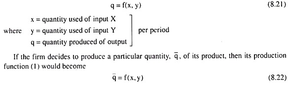
Taking total differential of the production function (8.21), we obtain

 

 

 

 

 

 

The second property of IQs that they are convex to the origin, follows straight from assumption (ii).

The third property of the IQs that they are non-intersecting, follows from assumption (v) which gives us MP_X, MP_Y > 0. In order to establish this property, let us suppose, for the sake of argument, that two IQs, viz., IQ₁ and IQ₂, have actually intersected at the point T in Fig. 8.6 and the points M and N are any two points on IQ₁ and IQ₂, respectively, N lying upward towards right of M.

Then we have output at M = output at T (M and T are on the same IQ, viz., IQ,) and output at T = output at N (T and N are on the same IQ, viz., IQ₂)

⇒ output at M = output at N.

But outputs at M and N cannot be equal because of assumption (v), since N, lying upward towards right of M, has more of both the inputs than M. Therefore, if any two IQs intersect (or touch) each other, then we arrive at a logical contradiction. Therefore, in our logical system the IQs must be non-intersecting.

Lastly, the fourth property of IQs that a higher IQ, i.e., one farther from the origin, represents a higher level of output, also follows from assumption (v). This is because a point on the higher IQ may be shown to lie to the north, east or north-east of some point on the lower IQ. But the reverse is not true.

That is, a point on the higher IQ may have either more of one input or more of both the inputs than some point on the lower IQ, but not the reverse. Therefore, because of assumption (v), a point on the higher IQ would represent a higher level of output than some point on the lower IQ. Hence the property follows. We may see in Fig. 8.7 that the points R, S and T on the higher IQ, IQ₂, lie, respectively, to the north, north-east, or east of the point A on the lower IQ, IQ₁.

Therefore, in the above discussion, we have seen that the IQs have four properties: they are negatively sloped, convex to the origin, non-intersecting and a higher IQ represents a higher level of output.

Two Special Types of Isoquants:

The IQs have four properties. These properties follow from some assumptions. The second of these assumptions is that substitution is possible between the two variable inputs used by the firm, but they are not perfect substitutes for one another—the MRTS_X,_Y diminishes as the firm uses more of input X and less of input Y. We may now see how the properties of IQs would be affected if we replace this ‘ordinarily’ made assumption by two uncommon or special assumptions, one by one.

(a) The First Special Assumption and the L-Shaped IQs:

If all other assumptions remaining the same, we replace the second assumption by the one that no substitution whatsoever is possible between the two inputs, i.e., the two inputs should always be used in a particular ratio, then the IQs would be L-shaped. We may obtain this in the following way.

Let us suppose that the required ratio between the two inputs is x : y = 1 : 1. In this case, if the firm can produce q, of output by using the input-combination (1, 1), then by using the combinations (1, 2), (1, 3), (1, 4), . . . , or, (2, 1), (3, 1), (4, 1), … , the firm would be able to produce the same qi of output.

For x remaining constant at x = 1 unit, if y is increased, or, y remaining constant at y = 1 unit, x is increased, then output would not increase. In this case, output would increase only when both the input quantities increase in the same ratio. For example, output produced by the combination (2, 2) would be larger than that produced by the combination (1, 1).

Now, it is obvious that if the combinations (1, 1), (1, 2), (1, 3), . . . , and (2, 1), (3, 1), (4, 1), . . . produce the same quantity of output q = q₁, then the IQ passing through these points would be L-shaped like IQ₁ in Fig. 8.9.

Similarly, if the output produced by the combination (2, 2) be q = q₂ (q₂ > q₁), then under the fixed ratio (here 1:1) case, the combinations (2, 3), (2, 4), (2, 5), . . . , (3, 2), (4, 2), (5, 2), … all can produce just the q = q₂ of output. Therefore, through all these combinations, we obtain the L-shaped IQ which is IQ₂, IQ₂ being higher than IQ₁. Similarly, for the combinations (3, 3), we obtain a still higher IQ like IQ₃, and so on.

Therefore, in our above discussion, we have seen that if the substitution between the two inputs is completely impossible, i.e., if the inputs are to be used in a fixed ratio, then the IQs would be L-shaped.

We may now take note of the following points: The numerical slope of the horizontal segment of an L-shaped IQ = 0. Therefore, at any point on this segment, MRTS_X,_Y = 0. On the other hand, at any point on the vertical segment of this IQ, the numerical slope = MRTS_X,_Y = ∞

We may obtain these values of MRTS in another way also. At any point on the horizontal segment of an L-shaped IQ, MP_X = 0 and MP_Y > 0. For if, at any point A on IQ₂, x increases from A to B, i.e., from 7 to 8 units, y remaining constant, then q does not increase—it remains the same at q = q₂, giving us MP_X = 0.

Again, at the point A, if x remaining the same, y rises from A to C, i.e., from 2 to 3 units, then q rises from q₂ to q₃, giving us MP_Y > 0. Therefore, at any point A on the horizontal segment of an L-shaped IQ, we have MRTS_X,_Y = MP_X/MP_Y = 0/+ ve = 0.

By similar reasoning, we would have MP_X > 0 and MP_Y = 0 at any point on the vertical segment of an IQ, giving us MRTS_X,Y = + ve/0 = ∞.

(b) The Second Special Assumption and the Negatively Sloped Straight Line IQs:

If all other assumptions underlying the ‘ordinary’ properties of the IQs remaining the same, we replace the diminishing MRTS assumption by a special assumption that the MRTS between the inputs is a constant, then the IQs would be negatively sloped straight lines.

This is because MRTS_{X Y} at any point in the input space being equal to the numerical slope of the IQ at that point, a constant MRTS implies that the IQs here would have a constant numerical slope. The slope of the IQ being negative, the IQs in this special case would be negatively sloped and parallel straight lines. We have shown some such IQs in Fig. 8.10.

In Fig. 8.10, we have assumed that the MRTS_X,Y = 2 = constant, i.e., the technology used by the firm is such that 2 units of input Y can always be substituted by 1 unit of input X. This implies that the slope of the IQs is -2 and the numerical slope is 2.