The Trade Indifference Curve: Assumptions & Properties | Economics

In this article we will discuss about the assumptions and properties of the trade indifference curve.

The device of trade indifference curve was originally forged by the writers like Leontief and Lerner. It was finally perfected by J.E. Meade in 1952 in his work, A Geometry of International Trade. This device shows, given a particular level of income, what terms of trade would leave a country neither better off nor worse off in respect of its international exchange with another country.

The trade indifference curve is the locus of such trade positions which are equally preferred for a country and, therefore, it is indifferent about them. In other words, a trade indifference curve represents those export-import combinations to which the given country is indifferent. Given a production possibility curve, a country can reach a certain commodity indifference curve and have a constant level of satisfaction, if the export-import combinations are prescribed by the trade-indifference curve.

Assumptions of Trade Indifference Curve:

It is possible to construct trade indifference curves on the basis of the following assumptions:

(i) There are two countries A and B dealing in two commodities—cloth and steel.

(ii) Cloth is A’s exportable and B’s importable commodity and steel is A’s importable and B’s exportable.

(iii) There are the conditions of perfect competition in the market.

(iv) There is an absence of external economies and diseconomies.

(v) The individuals in each country have identical tastes and factor endowments.

(vi) There is price flexibility that may lead towards full employment of resources.

(vii) The community indifference curves can be derived from the individual indifference curves and these are negatively sloped convex curves to the origin.

(viii) Given the factor endowments and techniques, the production possibility curve can be determined.

(ix) The production is governed by increasing costs so that the production possibility curve is a negatively sloping concave curve to the origin.

The trade indifference curve can be derived with the help of production possibility curve and the community indifference curve as shown in Fig. 4.4.

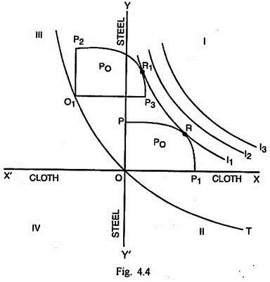
In Fig. 4.4, commodity cloth is measured along the horizontal scale XOX’. Cloth is A’s exportable and B’s importable. Commodity steel is measured along the vertical scale YOY’. This commodity is B’s exportable and A’s importable. I₁, I₂ and I₃ are the community indifference curves. PP₁ is the production possibility curve or opportunity cost curve. The area POP₁ represents the production block P₀.

The production possibility curve is tangent to the highest possible commodity indifference curve I₁ or R. This point indicates the quantities of cloth and steel consumed and produced in country A. If the production block P₀ is slided and origin shifts from O to O₁, the production possibility curve becomes tangent to the community indifference curve I₁ at R₁. Now point R) indicates the pattern of consumption and production. The points of origin O and O₁ can trace the path of the trade indifference curve T. Fig. 4.4 shows that the trade indifference curve slopes negatively.

On the basis of the procedure followed above, the trade indifference curves corresponding to the community indifference curves I₂ and I₃ can also be drawn. Along the same trade indifference curve, the country is indifferent between one and another trade position. Higher the trade indifference curve, the better off is the country and vice-versa. The trade indifference map of country B can similarly be drawn. The community indifference map of that country would be placed for that purpose in Quadrant III opposite to that of country A.

Properties of Trade Indifference Curve:

A trade indifference curve has the following main properties:

(i) For every community indifference curve, there is a corresponding trade indifference curve. The higher the community indifference curve, higher is the corresponding trade indifference curve and vice-versa.

(ii) The slope of the trade indifference curve at any point is equal to the slope of the corresponding community indifference curve and the production possibility curve at the corresponding point. It means the slope of T at O is equal to the slope of I₁ at R and the slope of T at O₁ is equal to the slope of I₁ at R₁ (Fig. 4.4).

(iii) If the community indifference curve is negatively sloped, the corresponding trade indifference curve is also negatively sloped.

(iv) If the community indifference curve is convex to the origin, the corresponding trade indifference curve is also convex to the origin.