The Offer Curve | Trade Equilibrium | Economics

For analysing the trade equilibrium of a country, another device that is employed is the Offer Curve or, more precisely, the Trade Offer Curve of a country. The trade offer curve indicates what quantities of a particular commodity one country are willing to offer in exchange of certain quantities of another commodity.

In other words, the offer curve shows the different quantities of a particular commodity demanded by one country from the other at the different relative prices of their products. It is because of this reason that the offer curve is known also as the reciprocal demand curve. The concept of offer curve was originally given by Marshall and Edgeworth.

For the derivation of the offer curve of a country, it is supposed that there are two countries A and B. Cloth is the exportable commodity of A (and importable of B), while steel is the exportable commodity of B (and importable of A). If the price of cloth continues to increase relative to the price of steel, the offer curve of country A can be derived as shown in Fig. 4.5 under constant cost conditions.

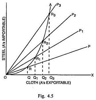
In Fig. 4.5, cloth (A’s exportable) is measured along horizontal scale and steel (A’s importable) is measured along the vertical scale. Originally the price ratio of two commodities is indicated by the slope of the line OP. If the price of cloth rises more relative to the price of steel, the slope of the price- ratio line or international exchange ratio line becomes more and steeper as shown by the lines OP₁, OP₂ and OP₃. As the price of cloth rises relatively more than steel, the demand for cloth in country B increases at a decreasing rate.

On the other hand, country A can absorb more quantities of steel at an increasing rate. If R, R₁, R₂ and R₃ are the points of exchange, the quantities exchanged between A and B are OQ of cloth and RQ of steel at R, OQ₁ of cloth and R₁Q₁ of steel at R₁, OQ₂ of cloth and R₂Q₂ of cloth at R₂ and OQ₃ of cloth and R₃Q₃ of steel at R₃. The additional quantities of cloth offered by country A decrease in exchange of the additional quantities of steel. By joining R, R₁, R₂ and R₃, it is possible to determine the offer curve OA of country A. It slopes positively at an increasing rate.

The derivation of the offer curve of country B is shown through Fig. 4.6.

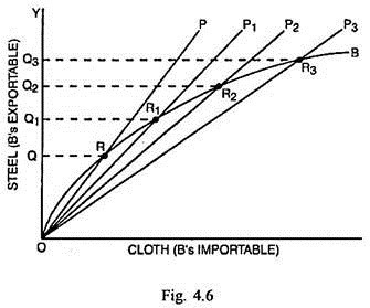
In Fig. 4.6, cloth (B’s importable) is measured along the horizontal scale and steel (B’s exportable) along the vertical scale. As the price of steel rises relative to the price of cloth, the steepness of the price ratio lines decreases. OP, OP₁, OP₂ and OP₃ are the price-ratio lines. Since the price of steel has been increasing at the greater rate, the demand for it in country A may increase at a diminishing rate.

The additional quantities of steel offered by country B become lesser and lesser given certain quantities of cloth offered by A. If exchange takes place at R, R₁, R₂ and R₃ points on the price ratio lines OP, OP₁ OP₂ and OP₃, the quantities offered are OQ, OQ₁, OQ₂ and OQ₃ of steel for the quantities of cloth RQ, R₁Q₁, R₂Q₂ and R₃Q₃ respectively.

By joining the points R, R₁, R₂ and R₃, the offer curve OB of country B can be determined. This offer curve also slopes positively at an increasing rate from the point of view of country B but at a decreasing rate from the point of country A.

Elasticity of Offer Curve:

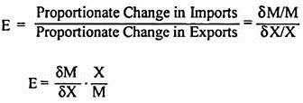
The concept of the elasticity of offer curve was coined by H.G. Johnson. The elasticity of offer curve is measured by a ratio of proportionate change in imports to proportionate change in exports.

The elasticity of the offer curve of two trading countries at specific points on their respective offer curves can be measured as shown in Figs. 4.7 and 4.8.

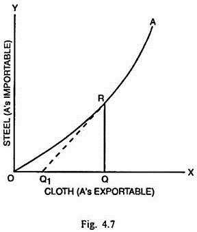
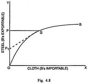
The elasticity of OA at R = (δM/δX) . X/M = (RQ/QQ₁) × (OQ/RQ) = OQ/OQ₁ > 1. To the right of point R, the offer curve becomes more and more elastic. The elasticity decreases as the exchange takes place to the left of point R. In Fig. 4.8, OB is the offer curve of country B.

The elasticity of OB at S = (δM/δX) . (X/M) = (PS/PP₁) × OP/PS = OP/OP₁ > 1.

The elasticity co-efficient, along this curve, decreases to the left of point S and increases to the right of point S.