
The following points highlight the top nine plan models used in Indian plans.
First Five Year Plan Model:
The estimate of the savings, in investment, capital output ratio, long term objectives along-with short term national income projections gives the idea that First Five Year Plan was based on the model of Harrod-Domar and it was set up in 1952.
Assumptions:
1. The marginal propensity to save is greater than the average propensity.
ADVERTISEMENTS:
2. The economy is closed.
3. The prices do not vary.
4. There is no difference between the marginal output capital ratio and the average capital output ratio.
According to this model the conditions of steady growth are:
The rate of investment iii the first five year plan was assumed to be 5 per cent of the national income, the value of capital output ratio is 3: 1 and the value of d was assumed to be 20%.
The investment was increased to 7 per cent in 1955-56, 11 per cent in 1960-61 and to 20 per cent of national income by 1967-68. If the growth rate of population was assumed to be 1.25 per cent per annum, the model demonstrates. “The proposed rate of marginal saving would cause no reduction in per capita consumption at any stage but would leave enough for a gradual rise in the consumption standards.”
The model based on the time lag of two years showed that the increase in investment and increase in output can also double the national income by 1971-72, the per capita income by 1977-78 and the average standard can be increased up to 70 per cent as compared with 1950-51.
The main drawback of this model was that it neglected the structural problems of the economy and it considered the development process as the rate of capital formation. The supposition of the constant marginal rate of saving ignored the problem of saving time. It did not take into account the real problems that the economy had to face in the development process. In short, there was little difference between the model and the actual planning process during the plan-period. However, it was merely an intellectual exercise.
Second Plan Model:
ADVERTISEMENTS:
The main architect of this model was Prof. P.C. Mahalanobis.
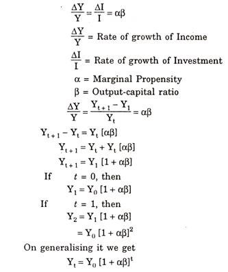
The mathematical equation of the model is as:
Yt = Y0 (1 + αβ – e)t
Y → National income per capita in year
α → Rate of investment
e → Rate of increase of population
β → Addition to national product which is generated by unit net investment.
Addition to national product which is generated by unit net investment.
The basic strategy was, “to increase investment in heavy industries and also on expenditure on services, to increase purchasing power and create fresh demand and on other hand, to increase the supply of consumer goods by increasing investment and production as much as possible in the small and household industries to meet the new demand.”
ADVERTISEMENTS:
He further writes:
“Planning would be thus essential feedback process of matching a continuously increasing demand by a continuously increasing production gives rise to a steadily expanding economy.”
The various assumptions on which model is based areas under:
1. The economy is closed with respect to foreign trade.
ADVERTISEMENTS:
2. There are no variations in prices during the plan.
3. The time lag between the period when investment is made and when actual production starts is one year.
4. Marginal utility of the consumption remains constant.
5. The capacity production in the consumer goods sector and capital goods sector is maximum.
ADVERTISEMENTS:
6. The supply of the capital goods determines the investment.
7. The rotation period of capital is constant.
8. Output capital ratios of the different sectors are independent of the capital labour ratio of those sectors.
9. The increase in the national income in one sector is not neutralized by some decrease in other sectors of the economy.
10. The products of capital goods sector can serve as input to the two sectors.
The plan used in Second Five Year Plan was divided in two Parts: Two Sector model and Four Sector model. In two sector model the economy is divided into two different sectors, the consumer goods sector ‘C’ and investment goods Sector ‘K’.
ADVERTISEMENTS:
The income growth path is given by following equation:
![]()
λk → Proportion of net investment in sector ‘K’
λc→ Proportion of net investment in sector ‘C’
βk → Output capital ratio in sector ‘K’
βc → Output capital ratio in sector ‘C’
ADVERTISEMENTS:
α0 →Initial rate of investment
Y0 → Income level in zero period
Y1 →Income level in period t.
In four sectors model was divided into four sectors:
1. Investment goods sector ‘K’
2. Factory produced consumer goods sector ‘C’
ADVERTISEMENTS:
3. Household produced consumer goods sector ‘C2‘
4. Services producing sector ‘C3‘
The income growth path equation of the Mahalanobis two sector model shows that income growth depends upon βk, βc, λk, λc and α0. In the initial stages the system grows at a slower rate but as the time passes the rate of growth increases. Due to this the Indian Planners laid great emphasis on investment in goods sector.
The growth model as contained in the second plan carried upto Fifth Five Year Plan (1975-76) as it is based on initial figures of First Plan. In 1961-70 the rate of growth of population was assumed to be 1.3 per cent. Capital Output ratio for the period of second plan was assumed to be 2.3: 1.
In 1955-56 the investment coefficient was 7 per cent which was expected to increase by 11 per cent in 1960-61. The marginal rate of saving was 0.2 and the increase in national income was estimated at 4.7 per cent by 1960-61 as against 2.5 per cent during first plan.
Third Plan Model:
The Third Five Year Plan consists of no specific plan model. It is simply based on the different relations expressed by Prof. S. Chakravarty in his famous article, “The mathematical Frame work of Third Model.”
ADVERTISEMENTS:
It consists of thirteen equations describing the various relationships:
1. The total investment is equal to the sum of the total domestic savings and net foreign aid i.e.
I = ∑It = ∑St + F
I → Investment
S → Saving
F → Foreign aid.
2. The net increase in the national income is equal to investment over whole period multiplied by output capital ratio i.e.
∆Y = β1
∆Y = Increase in investment
β= Output capital ratio.
3. Saving time at t is equal to the period of saving plus saving in period t
St = S0 + tα
α = Annual increase in national savings.
4. The demand for agricultural production depends upon the level of population as well as per capita income.
![]()
5. The increase in agricultural production is equal to investment in agricultural sector multiplied by capital output ratio.
∆YA = βAIA
6. The total tax revenue is equal to the autonomous tax revenue plus tax revenue which depends upon time.
It = nTt‘ + Tt”
7. The increase in the tax revenue is equal to the weighted average of the rates at which consumption, agricultural and non agricultural incomes are increasing.
![]()
8. Total govt. expenditure is equal to the sum of the current expenditure plus the proportion of total investment expenditure that is to be taken
∑E(t) = Ec(t) + Pil
9. Total increase in govt, debt is equal to the total expenditure minus total tax revenue and total amount of surpluses of pubic enterprises.
∆D = ∆Et – [∑Tt + ∑Rt]
10. Total increase in output is equal to the increase in agricultural output and the non agricultural output.
∆Y = ∆YA + ∆YNA
11. Total investment is equal to investment in agricultural sector plus investment in non agricultural sector.
12. Increase in output is either consumed or saved.
∆Yt = ∆C1 + ∆St
13. Increase in demand for agricultural goods is equal to increase in supply of agricultural goods.
∆DA = ∆YA
Now we have a set of thirteen equations and fifteen unknown. So this model is a ‘Decision Model’ as the number of unknown is more than the equations. So the value of two variables must be taken from outside arbitrarily and the remaining would be determined from the equation.
In this context Sandee observes, “Due to peculiar structure of the model, this simple target is wider than it seems. As investment and welfare go together, maximizing the one means maximizing the other. As gradual change has been assumed throughout, maximizing consumption and investment at the end of the period has the same effect as maximizing these two over the period as a whole.”
The third five year plan assumed the growth rate of population to be 2% per annum for the period 1961-71. The capital output ratio was assumed to be 23: 1. The saving rate increased from 8.5% in 1960-61 to 11.5% in 1965-66.
The Planning Commission stated that:
“If all the programmes included in the plan can be completed in time, national income at 1960-61 prices will go up by about 34%. Net output of agriculture and allied sectors will go up by 25%, of mining and factory establishments by about 82% and of other sectors by about 32%.”
Dr. V.V. Bhatta commented, “It was formulated without much regard to the choice possibilities either overtime or at a point of time. The project formulation and selection process as a result became somewhat arbitrary. The resulting imbalances and inefficiencies were further aggravated by deficiencies in the technique of planning and in actual operation of the policies which suffered from lack of coordination as well as meaningful operational link with development objectives.”
The assumptions of the third plan model were not fully achieved and they remained well below the targets.
Fourth Plan Model:
The plan model used in Fourth Five Year Plan was ‘Open Consistency Model’ prepared by Manne and Rudra with two different divisions of Planning Commission-the Economic Division and the Perspective Planning Division. It included 30-sector consistency model based on the conventional Leontief Inter Industry ‘Open’ system.
To show that the consistency of the model is ‘open’ rather than ‘closed’ type the first step is as under:
“It is to project the main components of gross domestic expenditure and to translate these into final demands for individual commodities. The model’s job is then to deduce an internally consistent set of sectorial output levels, imports and investment requirements. By working on an open one, we are in effect assuming that government has sufficient fiscal power so that it is unconstrained by the feedback link that operates in a market economy from the production process back to distribution of incomes, savings and generation of the domestic expenditures.”
The sectorial scheme has been expressed in triangular pattern of input dependence and at aims in the black angular structure of transactions matrix.
“The bulk of such transactions takes place within two virtually independent complexes; one based upon agriculture and the other upon mining, metals, machinery and forestry products. The first of these sectors is predominant source of consumption goods. The second is the source of investment goods and appears to be the strategic point for import substitution. A third and smaller complex produces items that may be described as ‘universal intermediates’-fuel, power, transport and chemicals-items are consumed within virtually all sectors of the economy.”
Manne and Rudra developed an inter-industrial matrix and also estimated the capital output ratio. They also made the demand projections. In 30 x 30 sector model out of 900 observations which were required, only in 240 non zero values were obtained.
For the Fourth Five Year Plan, Prof. Chakravarty, Prof Eckaus, Prof. Lefeber and Prof. Parekh discovered a temporal consistency model called CELP Model.
CELP Model:
This model is divided into eleven sectors:
1. Agriculture
2. Mining
3. Equipment
4. Chemicals
5. Cement and non-metals
6. Food, Clothing and Health
7. Electricity
8. Transport
9. Construction
10. Housing
11. Others
The statistical data was obtained from 30 x 30 model by Prof. Manne and Rudra. The main function of the CELP model was to indicate the sum of the consumption over the five year period.

t = Time
r = Social rate of discount.
The assumption of the model shows that consumption increases with respect to time does not fluctuate.
The main features of CELP model are as under:
1. It sums up the structural features of the preceding models making the preceding models as subcases of this model.
2. The development over time brought the economy from initial situation to the desired terminal situation.
3. It gives the clear idea of difference between investment at starting, investment in execution and completed investment.
The investments connected with social overheads and imports have been treated partly exogenously and partly endogenously. The macro variables like aggregate household consumption, government consumption and the exports have been treated exogenously.
Ashok Rudra showed that following lessons are yielded by this model:
1. The output of machinery and steel is primarily determined by the level of investment outlays, that of food-grains and cotton textiles taken wholly by the outlay or domestic consumption and that of petroleum products and electricity depend upon both.
2. The output levels of metal based industries are sensitive to assumption with respect to the import substitution programme, those of the other sectors are not.
3. The overall investment level is barely susceptible to the import substitution programme.
To get the investment rate, the consumption standard should be determined. The perspective planning division of Planning Commission showed that minimum standard of living would cost Rs. 35/- per person per month according to the prices in 1960-61. But only 20 per cent of the population in India enjoyed the living standard in 1960-61.
The remaining 80 per cent were below the poverty line. Therefore, the most important aim of the planning should be to raise the living standards so that even the poorest gets Rs. 35/- per month standard of living.
If this target was to be achieved by 1975, there should be 400 per cent increase in national income or annual rate of growth must be 10 per cent over the period of 1961-75 and as much as 12 per cent over the period 1966-75. The PPD recommended that if the data of achieving the goal were extended by another five years, then it would require rate of growth 8 per cent more than in 1966-1981.
The All Party working group – made following observations:
1. The national income of 5 persons should not be less than Rs. 100 per month i.e. Rs. 20 per person.
2. The expenditure provided by the state excludes the expenditure on health and education.
3. This target should be attained by 1975-76.
If the increase in national income is 7 per cent then the degree of inequality is unchanged during this period. Therefore, the PPD set the aim for fourth and fifth plan was that by getting 7 per cent growth rate during 1966-76 was to reach a national income of Rs. 20/-, per capita and for the people below 20 per cent, the government should take some special steps. The rate of 7 per cent increase in national income was less and to compensate this gap the national income target was raised to 7.5 or 7.7 per cent for fourth and fifth plans.
The technique which the PPD adopted was as follows:
1. To make projections at all macro levels.
2. The necessary material balances at micro level with lot of alterations are necessarily involved.
The first projection was made with the help of foreign trade. In fourth plan, it would be reduced considerably and in fifth plan it will be completely eliminated. The public consumption was made on the basis of targets of expansion in education, health and other social services.
The rate of investment was expected to increase by 21 per cent and tends to remain the same for next five years. The personal consumption was derived from deducting the sum of projected level of expenditure on investment and public consumption from gross domestic expenditure.
The next step was to work out the “broad commodity pattern for the gross domestic demand at various points of time.” The calculations showed that the consumption was to reach 210.3 Abjas where 1 Abja = 100 crores.
The changes in the consumption pattern and the rise in consumption level is derived on the account of elasticities for individual items of consumption were assumed from NSS data. Similarly, the commodity pattern of public consumption was achieved by using suitable techniques of projections.
The income generated represents the sum of wages, salaries, interests and the profit earned by various factory owners. It can be easily shown that if income generated from different commodities are taken together it would give the national income. The target for sectorial incomes and national income given by PPD are not some adhoc figures spun out of nothing.
The PPD presents a large number of articles regarding material balances at micro level. A material balance for a commodity is the demand for that particular commodity originating in all major industries in which the commodity is used along with the indication how the total required quantity of commodity is proposed to be produced in the country or imported from the abroad.
The material balances indicated by PPD were coal, petroleum products, electricity, iron ore, manganese ore, lime stone, china clay, gypsum, bauxite etc. If we take the details of the plan it provides more opportunity for the job of engineers and technicians rather than economists or statisticians. This is the main reason that the staff of PPD is of engineers and technicians.
This plan represents the separate figure for the financial variables and estimated for the terminal year of the plan. The link between the macro plan and the financial plan was established by matching the needs of investment with the source of supply. This model can be used to calculate the time path for variables such as consumption, production and investment.
The main drawbacks which admitted by the authors itself were as follows:
1. Richard S. Eckaus admits that the assumption of linearity is “an unfortunate restriction.” According to him, “The use of a composite good as a consumption variable is undoubtedly a major obstruction.”
2. The increased employment and the improved income distribution are the important aims of the plans, but they are not fully achieved.
3. A number of planning decisions for which alternatives are worth considering have been left outside.
4. Input coefficients are taken as constant but these must change according to the structural changes in the economy.
5. Srinivasan raised that the terminal conditions in the model are laid down to sustain post terminal growth rates of consumption where the composition of consumption is determined exogenously, but its scale is left to be determined by optimising mechanism.
Fifth Plan Model:
The fifth plan model is based on the “Technical Note on the Approach to fifth plan of India 1974-79” prepared by the Perspective Planning division of Indian Planning Commission. It is multi sector, modified open ended static input output model. Its main aim is to remove poverty and attain self reliance by 1979.
According to Suresh D. Tendulkar, “It can be traced to certain basic inadequacies in institutional specification of the model as well as certain inherent rigidities in it, certain pronounced bases in the parametric specifications and the absence of a policy frame to back up the quantification of social objectives in the Approach document.”
For a given set of input output coefficients and the sectorial levels of final demand for the terminal year, the model provides a consistent set of sectoral targets of gross output.
The pattern of utilization of total supplies from domestic production and imports for the sector in period is written as: 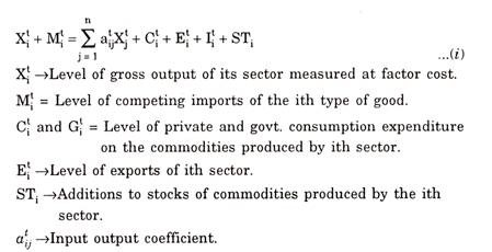
This model was formulated by considering the technological characteristics of the economy as reflected in inter industry relationship. It involves input output matrix and elaborate system of internal balances. It was a macro-economic 66 sector input output model with a consumption sub model.
The production levels were estimated by their demand supply balances through a series of exercises of material balances and making them consistent with sectoral growth rates of input output model. The consumption proportion matrices were based on consumer expenditure data by commodities of 25th Round of National Sample Survey as well as the estimates of private consumption expenditure on different commodities. A 10% growth of public consumption was assumed and exports were estimated to increase at the rate of 8.55 per annum.
In 1979, when plan was to end, private consumption and imports were estimated endogenously by making following specifications:
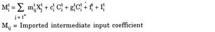
Cti, gti, fti →Coefficients indicating the requirement of competing imports of the ith type per unit of private and government consumption and gross fixed investment respectively.
Putting these values in equation 1 we get
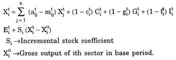
Thus the above equation provides a system of n simultaneous equations one for each sector, which when solved, provides for terminal year of the plan a set of sectoral targets. The total investment laid for fifth plan had been appropriately achieved in the plan period.
The total investment estimated to be financed from domestic sources was 91 percent. Of the aggregate investment about 58 percent was achieved in public sector and 42 percent in private sector.
The 27 percent of the domestic savings were to be contributed by public sector and the rest 73 percent were to come from private sector consisting of corporate savings and cooperative and household savings. The average rate of domestic saving was expected to rise from 14.4 percent in 1973-74 to 15.9 percent in 1978-79.
Public savings were estimated to grow from 2.5 percent of GNP in 1973-74 to 11.3 percent in 1978-79. The overall annual rate of growth had been approximated 4.37 percent as against 5.5 percent given in both the Technical Note and Draft Plan.
The growth rate of output in agriculture sector was 3.94 percent per annum of mining and manufacture 7.10 percent, electricity 10.12 percent, construction 5.90 percent, transport 4.79 percent and of services 4.88%. The share of agricultural sector was decreased from 50.78 percent in 1973-74 to 48.15 percent in 1978- 79 while the share of mining and manufacturing was estimated to increase from 15.78 to 17.49 percent.
The marginal increase in electricity; transport construction and services were also obtained. The projected rate of growth were translated into physical targets. For items like coal, crude oil, iron ore and cement which formed independent sectors in input output model, targets have been taken out directly from sectoral growth rates. In other cases, material balances and other planning exercises were employed.
The planning exercises deal with two variants:
1. Unchanged Quality.
2. Postulated reduction inequality coefficient.
The pattern of growth rates of output in core sectors of the economy which provide infra structural facilities which were largely invariant with respect to any alterations in the inequality parameter for luxury consumption sectors, the preferred variant imposed more vigorous curbs on their growth.
The draft fifth of five year plan kept the suggestion of the removal of poverty and attainment of self reliance. As noted by Tendulkar, the basic statement of the removal of poverty as contained in Draft Fifth plan was a vague statement.
The remedies done to remove poverty were not effective and have their quantitative effects on the attainment of the social objective of the changes in the institutional frame work were given in non operational terms such as ‘attitude transformation’ and ‘structural reformation.’
Sixth Plan Model:
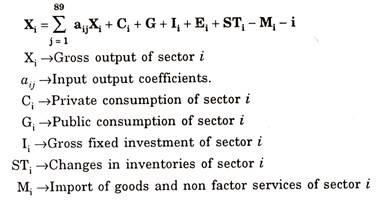
The sixth plan model was based on the ‘Technical Note of the Sixth Plan’ prepared by the Perspective Planning Division of the Planning Commission. The macro structure of the model had been prepared on 89-sector classification of input output table. It closely resembles with fifth plan mode. This plan model consists of core models and several sub models. The sub models are designed to provide necessary input to the core models.
Core model consists of following things:
1. Input output
2. Investment
3. Private consumption
4. Financial resources
5. Import
6. Employment
7. Perspective Planning
Sub models taken are as under:
1. Agriculture
2. Exports
3. Demography
4. Autonomous investment
5. Long term objectives.
The analytical model comprises an input output model, a macro economic model and consumption sub model.
It is of the static Leontief type:
Mathematically the model is as follows:
The model system covers a 15 year period from 1980-81 to 1994-95 in two sub periods:
(i) Medium term of 5 year period from 1980-81 to 1984-85 conceding with Sixth Five Year Plan.
(ii) Long time span of 10 years 1985-86 to 1994-95 defined by long perspective plan.
To attain the required objectives the rate of growth 5.2 percent in sixth plan and 5.5% percent in next ten years. For this, it used a large number of social and economic indicator as GDP at 1979-80 prices, consumption, saving, investment, employment, per capita income and consumption number of the people below poverty line.
The population projections were made to estimate the demand for goods and services and employment. The annual average growth rate of population was 1.79 percent during 1981-86, 1.66 percent during 1986-91 and 1.55 percent in 1991-96.
The plan model has done a lot to reduce the percentage of population below poverty line to 30 in 1984-85 and to less than 10 by 1994-95. The net increase in employment, measured in standard person at the rate of 3.4 percent per annum against a labour force growth of 2.4 percent per annum.
The development strategy of the plan found a change in the existing structure in favour of investment and social consumption. The rate of capital formation was increased from 21.5% percent of GNP for 1979-80 to 25 percent in 1984-85 and the public consumption was increased from 10.7 percent of GNP in 1979-80 to 11.5 percent in 1984-95.
“The rise in the share of domestic capital formation as well as that of public consumption, together with the projected improvement in export, implies a decline in the share of private consumption in gross national expenditure.” Due to this decline the private consumption expenditure was estimated to grow at a rate of 4.7 percent during 1980-85.
The rate of saving had been increased from 21 percent of GNP in 1979-80 to 24.4 percent in 1984-85. The growth in domestic saving was to be achieved through rise in ratio of saving to disposable income of both public and the private sectors.
The output of the agricultural sector grew at an annual rate of 5.2 percent during 1979-80 to 1984-85, of mining and manufacturing at 7.76 percent, electricity and water supply at 11.25 percent, transport6.7 percent and services 6.70 percent over the period.
“The varying rates of growth in different sectors reflected the changes in the rates of growth of total final and intermediate demand for output of different sectors which were themselves influenced by factors like degree of import dependence, relative changes in composition of final demand, inter-industry relationships etc. The rates of growth estimated for different sectors were also expected to bring about a structural change in the economy as reflected in the composition of GDP at factor cost over prospective period.”
As far as the objective of removal of poverty is concerned both the fifth and sixth plan stated the minimum need objective in private consumption through the concept of poverty line. The fifth plan targeted to raise the per capita expenditure of the lowest 30 percent of population upto the poverty line in terminal year so that only 15 percent of people were left below poverty line.
The sixth plan presented a modest target leaving 30 percent of people below the poverty line in its terminal year i.e. 1984-85. The share of agriculture was projected to decline from 35.13 percent in 1979-80 to 32.9 percent in 1984-85. The growth rates were adjusted such that total plan investment for all sectors combined which lies within the limit put by financial resource working group. The main objective of the plan was to increase the rate of growth removing the constraints.
The Technical Note mentions three main fractures of sixth plan:
1. A system of supply equations which is an extended and modified version of Harrod Domar equation, meant to accommodate sectoral dis-aggregations, questions of investment gaps and existence of a foreign trade sector.
2. A system of demand equation which is an extended version of Leontiefs input output system by endogenising not only consumption and imports but also investment.
3. A set of inequality relations with given upper bounds as Mx < R to ensure that demand should not exceed the supply in any of the markets dealing with commodities services, capital labour, foreign exchange and renewable sources. In the same way the set of an inequality relations with lower bounds given as M* x* = R* were used to ensure the attainment of minimum welfare targets of community.
Seventh Plan Model:
The macro and sectoral structure of seventh plan is basically originated from sixth plan mode. The macro structure of the model is based on the 89-sector classification of input output table which is classified into 50 sectors. In 1984-85 the rate of domestic savings was 23.3 per cent of GDP and which was expected to rise 24.5 per cent in 1989-90.
From here we can conclude that the rate of marginal savings is 28.4 per cent. The broad quantitative concept of the plan was based on the estimation of overall ICOR of 5. The rate of gross investment was assumed to rise from 24.5 per cent of GDP to 25.9 per cent from 1984-85 to 1989-90.
The rate of growth of agricultural output is estimated to be 4 percent of minerals and industrial goods at 8.3 per cent, electricity, water supply and gas at 12 per cent, of transport at 8 per cent and other services at 6.6 per cent. The sectoral composition of national income had been estimated.
The share of agriculture and related sectors was projected to be 33 per cent of GDP in terminal year of Seventh Plan. The contribution of mining, manufacturing, construction, electricity and transport were projected to be 34.4 per cent. Thus by the end of the plan the income generated by industrial sector, agricultural sector and service is one third of each sector.
The Eight Plan Model:
The model in Eighth Plan was based on “A Technical Note to the Eighth Plan of India 1992-97” prepared by the perspective Planning Division of the Planning Commission. The analytical model consisted of a macro-economic model, an input model, an investment model and five sub-models relating to agriculture, industry, trade, consumption and financial resources.
The macro-economic model was a set of structural equations relating to such macro variables as GDP at factor cost, GDP at market prices, GNP, gross domestic savings, gross fixed investment, disposable income, total consumption, exports of goods and non-factor services and imports of goods and non-factor services. Some variables like consumption and exports were determined exogenously while imports and savings and investment were determined endogenously.
The macro structure of the Plan had been prepared on the basis of 115 sector classification of the input output table which was aggregated to 60 sectors. The input-output tables were adjusted to the levels and structure of prices in 1991-92.
The investment model was based on a stipulated level of output. It has two components: Investment by destination and investment by source or origin. To estimate investment by destination an econometric simulation model was used which was then converted into investment by source with the help of a capital coefficient matrix. Then, estimates were included in the input output matrix.
Given the overall targeted growth rate of the economy during the Plan, the sectoral pattern of output and related growth rates were obtained through the consistency model. The consistency model began with the final demand and took into account inter-sectoral linkages through inputs and outputs.
The main components of the final demand were: private final assumption, government final consumption, saving investment, exports were determined exogenously, saving, investment and imports were determined endogenously in the model. Each one of these components was worked out through a sub-model. Each sub-model was based on the dominant parameters obtained from analysis of past data.
Based on the calculations of the model, the sectoral growth rates for the Eighth Five Year Plan were projected at gross value added at factor cost. On this basis, the overall growth rate of the economy was estimated at 5.6 percent per annum. The envisaged sectoral annual growth rates for Plan were: agriculture 3.1 percent, mining 8 percent; manufacturing 7.3 percent, electricity, gas and water 7.8 percent; construction 4.7 percent; transport 6.7 percent; communication 6.1 percent; and other services 6 percent.
These estimates were based on the assumption that during the Plan period ICOR would be 4.1; average domestic savings 21.6 percent per annum; the rate of average annual investment 23.2 percent; current account deficit 1.6 percent of GDP; the growth rate in export of goods 13.6 percent and the growth rate in import of goods 8.4 percent per annum.
On the basis of these, a total investment of Rs. 7, 98,000 crores at 1991-92 prices had been envisaged for the Plan period, and the total outlay for the public sector had been fixed at Rs. 4.34,100 crores, i.e., 45.2 percent of total investment.
The Eight Plan model also drew a perspective plan covering a period of 15 years from 1991-92 to 2006-07. This long-term development perspective visualised the long-term needs of the society and the directions in which the economy should move over a longer time horizon.
To determine the long-term conditions of growth, it analysed the demographic trends, the basic resource endowment, the entrepreneurial resources and the technology perspective.
For working out the long-term growth perspective, the projections for the terminal year (1996-97) of the Eighth Plan were taken in respect of the various macro parameters and sectoral output levels. These were calculated on the basis of the same macro- economic model, input-output model and consistency model used for the main Plan projections.
Some projections of macro parameters of growth were: the annual average GDP growth rate of 5.6 percent during 1992-97, 6.05 percent during 1997-2002, and 6.51 percent during 2002-07; average annual saving rate of 21.6 percent, 23.2 percent and 24.4 percent respectively; average annual investment rate of 23.17 percent, 24.2 percent and 25.4 percent respectively; and average annual growth rate of total consumption of 5.6 percent, 5.62 percent and 6.18 percent respectively. These projections were based on the assumption of ICOR of 4.1 for the Eighth Plan and 4 and 3.9 respectively for the periods 1997-02 and 2002-07.
The Ninth Plan Model:
The Ninth Plan, 1997-2000 is based primarily on the Eighth Plan Model.
In calculating its parameters, the following specific assumptions were made:
(i) The base year of the Plan was taken as 1996-97.
(ii) Calculations were made at 1996-97 prices.
(iii) Trends in public and total domestic savings witnessed in the last couple of years would continue.
(iv) Major contribution to public savings would come from Government’s performance by: (a) improving taxes net of subsidies, and (b) maintaining the share of public consumption expenditure in GDP more or less at the same level.
(v) Total public investment was determined to achieve a fiscal deficit target of 4 per cent for the Centre during the Plan period.
(vi) ICOR would tend to rise to 4.3 during the Plan due to emphasis on investment in infrastructure. This parameter was generated by the model to ensure that the growth rate of the economy would not suffer in the post-Plan period due to infrastructure bottlenecks arising from shortfalls in pipeline investment.
On the basis of the above cited parameters, the Perspective Planning Division of the Planning Commission presented two growth scenarios envisaging (i) a projected GDP growth rate of 6.2 percent per annum, and (ii) an accelerated GDP growth rate of 7 percent per annum for the Plan period. Since there was delay of about two years in finalising the Plan document, the Plan model was reworked with the growth target of 6.5 percent per annum on an average.
The revised and final macro parameters consistent with the targeted GDP growth rate of 6.5 percent for the Ninth Plan are: average domestic savings rate of 26.1 percent per annum; average annual investment rate of 28.2 percent; current account deficit 2.1 percent of GDP; export growth rate of 11.8 percent per annum; import growth rate of 10.8 percent per annum.
The estimate of current account deficit is base on the assumption that the increase in foreign exchange reserves would be 0.2 percent of GDP and the total external inflow 2.3 percent of GDP during the Plan period.
The sectoral pattern of growth envisaged for the Ninth Plan and the associated ICORs have been generated from the Plan model by imposing exogenously determined growth targets for the various sectors and taking into account all the relevant leads and lags.
Accordingly, the envisaged annual sectoral growth rates for the Plan are : agriculture 3.9 percent ; mining 7.2 percent ; manufacturing 8.2 percent ; electricity, gas and water 9.3 percent; construction 4.9 percent; trade 6.7 percent ; transport 11.3 per cent, communications 9.5 percent; financial services 9.9 percent ; public administration 6.6 percent; and other services 6.6 percent.
These estimates are based on the aggregate ICOR of 4.3 with high sectoral ICORs in the case of infrastructural sectors. These estimates have been made on the basis of the sectoral consistency demand-supply model which took into account final demand, inter-sectoral transactional demand, export possibilities, import intensities and the overall availability of investible resources.
The main objectives of the Ninth Plan being Growth with Social Justice and Equity, the Plan model worked out the population growth rate of 1,57 percent and of the labour force 2.85 percent in the terminal year of the Plan. Based on these projections with the average annual growth rate of 6.5 percent for the economy, the unemployment rate was estimated at 1.8 percent.
At the end of the Plan, the per capita household consumption was projected to grow at 4.3 percent per year. This was derived from the estimated annual growth rates of food-grains (3.2 percent), other food (5.8 percent) and non-food (7.5 percent).
The household component of consumption in the base year and terminal year of the Plan was flowed through a vector of state-wise consumption proportions to allocate the total consumption among the states.
This vector was obtained from the growth in total consumption of each state between 1983-84 and 1993-94 (assumed unchanged) relative to the growth in total national consumption.
The State-wise household consumption component so derived was broken up into rural and urban components on the basis of urban-rural per capita consumption differentials as given by the per capita urban-rural expenditure data of 1993-94, assumed as unchanged.
From the state-wise distribution functions of consumption expenditure, the state-specific estimates of poverty for the Ninth Year Plan were worked out using state specific poverty lines computed as per the methodology of the Expert Group. The poverty ratios were worked out separately for each state in rural and urban areas.
The estimate of national level poverty ratio in rural and urban areas was computed as the weighted average of state poverty ratios as per the Expert Group methodology. In the incidence of poverty in rural and urban areas at the national level was also worked out from the national level consumption distribution of the NSS and national poverty line.
Accordingly, the Ninth Plan model estimated the incidence of poverty in the terminal year of the Ninth Plan as 18.61 percent in rural areas, 16.46 percent in urban areas and 17.98 percent for the country as a whole.
To achieve the above mentioned sectoral and overall growth rates and the principal objective of the Plan, the aggregate public outlay for the Ninth Plan has been worked out to Rs. 8,59,200 crore at 1996-97 prices.