Game Theory I : A Close View

let us make an in-depth study of the game theory I in economics.

Subject-Matter of Game Theory I:

Game Theory is the study of strategic interactions between players.

These occur frequently within economics, as well as in the rest of the world. Oligopolies present one of the most common areas where game theory is used within economics.

Other areas include bargaining and auction theory. Game theory can also be used in some labour market theories and in the financial markets. Any decision which involve choice can be modelled using game theory.

We will look at game theory in two stages. Firstly, we will look at the basic tools and models. Secondly, we can apply our game theory knowledge to several areas of microeconomics, e.g., oligopoly ideas.

Prisoners’ Dilemma:

Consider that two people who have been imprisoned by the authorities who have kept them in separate cells, but with little evidence to convict them. They tell each person that the other one has confessed to the crime, and that he should do the same to make the best of a bad situation.

If both people confess they get 6 years in jail. If only one confesses, he gets 1 year and the other gets 9 years. If neither confesses, they each get 2 years.

Now each person has to choose whether or not to confess. If the other person has confessed, then by not confessing they get 9 years, whereas, by confessing they get 6 years. If the other person has not confessed, then by not confessing they get 2 years, whereas, by confessing they get 1 year.

It is clear that it is best, in either case, to confess. Thus, the outcome will be that they both get 6 years, since they both make the same decision.

In this explicit format the problem is not easily recognised as the prisoners’ dilemma, and so a format called a ‘bi-matrix’ has been developed. In the scenario described of each, the prisoners make their choices simultaneously. They each decide whether or not to confess.

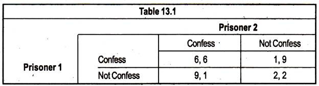
In this case, we can see that if prisoner 2 is going to confess, then it is best for prisoner 1 to confess. If prisoner 2 is not going to confess, it is still best for prisoner 1 to confess. Thus, it is best for prisoner 1 to confess regardless of what prisoner 2 does and this confession is his dominant strategy. The situation is exactly the same for prisoner 2. The dominant strategy is defined as one that is optimal for a player, no matter what an opponent does.

Example of dominant strategy in a duopoly setting:

Suppose Firms A and B, selling, competing products, are deciding whether to undertake advertising campaigns. However, each firm will be affected by its competitor’s decision.

The possible outcomes of the game are illustrated by the payoff matrix in Table 13.2 below:

This payoff matrix shows that if both firms decide to advertise, Firm A will make a profit of 10, and Firm B will make a profit of 5. If Firm A advertises and Firm B does not, Firm A will earn 15, and Firm B will earn zero. And, similarly, for the other two possibilities. What strategy should each firm choose? First, consider Firm A.

It should advertise because no matter what Firm B does, Firm A does best by advertising. Thus, advertising is a dominant strategy for Firm A.

The same is true for Firm B. No matter what Firm A does, Firm B does best by advertising. Thus, assuming that both firms are rational, we know that the result for this game is that both firm will advertise. This outcome is easy to determine because both firms have dominant strategies.

However, many games do not have a dominant strategy for each player. Let us examine the payoff matrix given in the table below, which is the same as the above matrix, except for the bottom right-hand corner, if neither firm advertises, Firm B will again earn a profit of 2, but Firm A will earn a profit of 20.

Now Firm A has no dominant strategy. Its optimal decision depends on what Firm B does. If Firm B advertises, then Firm A does best by advertising; but if Firm B does not advertise, Firm A also does best by not advertising. Now suppose both firms must make their decisions at the same time. What should Firm A do?

To answer this, Firm A must put itself in Firm B’s shoes. What decision is best from Firm B’s point of view, and what is Firm B likely to do? The answer is that Firm B has a dominant strategy, to advertise, no matter what Firm A does. Thus, Firm A’s conclusion is that Firm B will advertise. This means that Firm A should also advertise. The equilibrium is that both firms will advertise.

We can see that the Nash Equilibrium of the prisoner’s dilemma is not Pareto efficient, since if they both do not confess, they are both better-off than the dominant strategy outcome. This situation will form the basis of many economic situations  with the options of confessing and not confessing being replaced by high price, low price or high output, low output and the two prisoners being replaced by oligopolistic firms.

This situation can also be applied to several other problems, including warfare, where the options of confessing and not confessing can be replaced by deploying or not deploying missiles. In either case, the country is best served by deploying missiles.

Nash Equilibrium:

To determine the likely outcome of a game, we have been seeking a “stable-equilibrium”. Dominant strategies are stable, but, in many games, dominant strategies do not exist, so, we need to be able to analyse games which do not have dominant strategies.

We need a more general equilibrium concept. Thus, we introduce a Nash Equilibrium as a set of strategies such that each player is doing the best it can, given the actions of its opponents.

Since each player has no incentive to deviate from a Nash Equilibrium, the outcome is stable. In the second advertisement example, the Nash Equilibrium is that both firms advertise. It is a Nash Equilibrium because, given the decision of its competitor, each firm is satisfied that it has made the best possible decision, and has no incentive to change its decision.

Consider the game below:

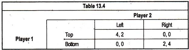
The best that player 1 can do, given that player 2 has played left, is to play top. We call this pair of strategies a Nash Equilibrium. Similarly, bottom, right is also a Nash Equilibrium (NE). This concept was formalized since dominant strategies are often difficult to find or may not exist. However, the NE of a game depends on what both players do.

We can say that a pair of strategies can be called a Nash Equilibrium if A’s choice is optimal given B’s choice and B’s choice is optimal given A’s choice. The Nash Equilibrium of the prisoners’ dilemma in Table 13.1, described above is (Confess, Confess). The NE of a game is the generalisation of the Cournot Equilibrium for oligopolies, where each firm maximises its own payoff, given the other firm’s actions.

It is helpful to compare the concept of a Nash Equilibrium with that of an equilibrium in dominant strategies:

Dominant Strategies:

I am doing the best I can, no matter what you do. You are doing the best you can, no matter what I do.

Nash Equilibrium:

I am doing the best I can, given what you are doing. You are doing the best you can, given what I am doing.

Note that a dominant strategy equilibrium is a special case of a Nash Equilibrium.

In the advertising game of Table 13.3, there is a single Nash Equilibrium — both firms advertise. In general, a game does not have to have a single Nash Equilibrium. Sometimes there is no Nash Equilibrium, and sometimes there are several.

Consider the “Production Choice Problem” of two firms, in Table 13.5.

Example of two Nash Equilibrium:

In this game, each firm is indifferent about which product it produces, so long as it does not introduce the same product as its competitor. If coordination were possible, the firms would agree to divide the market. Suppose that somehow Firm 1 indicates it is about to introduce the sweet cereal, and Firm 2 indicates it will introduce the crispy one.

Now, given the action it believes its competitor is taking, neither firm has an incentive to deviate from its proposed action. If it takes the proposed action, its payoff is 10, but if it deviates, its payoff will be -5, given that the competitor’s action remains unchanged. Thus, the strategy set given by the upper right-hand or bottom left-hand corner of the payoff matrix is stable and in Nash Equilibrium.

Each Nash Equilibrium is stable, because, once the strategies are chosen, no player will unilaterally deviate from them. Both firms have a strong incentive to reach one of the two Nash Equilibria — if they both introduce the same type of cereal, they both lose.

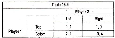
There may be games without Nash Equilibrium, as in Table 13.6.:

Maximin Strategies:

The concept of a Nash Equilibrium relies on individual rationality. Each player’s choice of strategy depends not only on his own rationality, but, also, on that of his opponent. This can be a limitation, as the example of Table 13.7 shows.

In this game, playing right is a dominant strategy for player 2, because, this strategy will be better for player 2 (earning 1 rather than 0), no matter what player 1 does. Thus, player 1 should expect player 2 to play this strategy. In this case, player 1 would do better by playing bottom (earning 2) than by playing top (earning 1).

Clearly, the outcome — bottom right — is a Nash Equilibrium for this game, and this is the only Nash Equilibrium for this game. But player 1 should be sure that player 2 understands this game and is rational. If player 2 should happen to make a mistake and play left, it would be extremely costly to player 1.

If you were player 1, what would you do? If you tend to be cautious, and are concerned that player 2 might not be fully informed or rational, you might choose to play top, because, this is the safe strategy. Such a strategy is called a maximin strategy because it maximises the minimum gain that can be earned.

If both players used maximised strategies, the outcome would be (top, right), a maximin strategy is conservative, but not profit-maximising. Note that if player 1 knew for certain that player 2 was using a maximin strategy, he would prefer to play bottom, instead of playing the maximin strategy of playing top.

Mixed Strategies:

Choosing a pair of strategies as a Nash Equilibrium can be further generalized to include what we call mixed strategies. This is when a player can choose between pure strategies in a certain proportion. For example, a mixed strategy is to play top 70% of the time and bottom 30% of the time. In these terms, a pure strategy is a mixed strategy, where one option has a weight of 100%.

A Nash Equilibrium in mixed strategies, therefore, refers to an equilibrium in which each agent chooses the optimal frequency with which to play his choices, given the frequency of choices by the other player. It can be shown that in most games, there exists a mixed strategy Nash Equilibrium.

The above game has a Nash Equilibrium when player 1 plays top with probability 3/4 and bottom with probability 1/4, and player 2 plays left or right with a probability of 1/2.

Repeated Games:

So far we have only dealt with games that are played once. However, in reality, many games are played more than once. For example, a firm in an oligopolistic industry will choose its price each month, or choose its output each month, or at some other interval.

This, in effect, means that the same game is played over and over again. We will look at the case of repeated games for prices in an oligopoly. The outcome depends on two things. Firstly, whether opponents will punish defectors who play a Pareto inefficient choice. Secondly, on whether the number of times the game is to be played is fixed or infinite.

Let us consider the game (given on page 224) being played 10 times. In the final round, neither player has an incentive to cooperate and, thus, it is best for each player to defect and lower prices. Therefore, in round 9, the players know that the other will defect in the next round and, thus, there is no incentive to cooperate in round 9.

We can go back in the same manner, showing that there is no incentive to cooperate in any round and, thus, the Nash Equilibrium is to defect.

This can be shown to be the case for any prisoners’ dilemma game with a fixed number of games. Since there is no possibility of further play in the last round, it is best to defect. But, then, why should players not defect in the penultimate round? Or the one before that? And so on.

However, if the game is played an infinite number of times, then one player can influence the other’s choices, given that each player values future payoffs enough. Consider the strategy that you begin by cooperating in the first round.

Then, in subsequent rounds, you play whatever your opponent has played in the previous round. Thus, if they have defected, you punish them in the next round. If they have cooperated, you continue to cooperate.

This strategy is known as ‘tit for tat’ and has been shown by Robert Axelrod to give the best outcome in an infinitely repeated prisoners’ dilemma game. This is because both players learn quickly that defecting is punished by immediate retaliation and, thus, in the long-run it is best to cooperate, and this result can be seen in many cartels that operate in the world today.

Sequential Games:

Until now we have only considered games where the players play at the same time. However, there are many important areas when one player plays before the other. The Stackelberg model, is an example of a sequential game.

Let us describe a game where there are two rounds. In the first round, player 1 chooses top or bottom. Then; in the second round, player 2 chooses left or right.

The payoff bi-matrix is as follows:

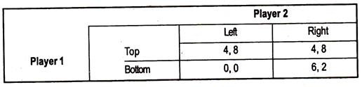
In this form, we can see that both top, left and bottom, right are Nash Equilibria, but we will show that one of these is not really reasonable. To do this we need to picture the game in a game tree format or extensive form. This form shows more clearly the asymmetric nature of the game, where one player chooses before the others.

The game in extensive form is as follows:

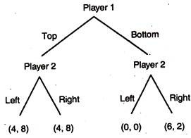
We solve this game by analysing backwards. This is often referred to as backward induction or Zermelo’s algorithm. If player 1 has played top, then it does not matter to player 2 what he plays, since his payoff is 8 and player 1 gets 4. If player 1 has played bottom, then player 2 is better-off playing right since this gives him a payoff of 2 as opposed to 0 from playing left.

Player 1 knows this and, thus, chooses between a payoff of 4 from playing top and 6 from playing bottom. He chooses bottom and, thus, we have shown that bottom, right is the only reasonable Nash Equilibrium in this game.

This outcome is clearly not as good for player 2 as the outcome from top, left. Player 2 can only influence the outcome, if by some means he can convince player 1 that if he plays bottom, player 2 will play left even though this hurts him as well. The problem is that, once the decision time for player 2 is reached, it is optimal for him to play right and, thus, the credibility of the threat is eliminated.