How Wages are Determined under Non-Pure Competition? | Economics

The following article will guide you about how wages are determined under non-pure competition.

Wage is the price of labour as a factor. In a competitive labour market, the wage rate, like the price of any commodity, is determined by the market forces, i.e., by the forces of demand and supply. Each individual worker acts as a price-taker, i.e., takes the prevailing wage rate as given, and decides how much labour service to supply at that wage.

Each worker has a supply curve showing how much labour power (in terms of hours worked) he (she) will supply at each wage. By adding up these individual labour supply curves, we arrive at a market supply curve which shows the total supply of labour (in terms of labour hours) to this market as a function of the real wage.

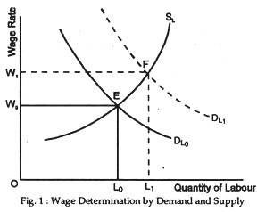
Likewise, on the demand side of a competitive market there are so many purchases of labour power that no one of them can exert any influence on the market wage rate. Instead, each employer just decides how much labour to hire at the current rate. Since in a perfectly competitive market both demanders and suppliers are price-takers and quantity-adjusters, the wage-rate and the volume of employment is determined by the forces of demand and supply as is shown in Fig. 1. Here, the original de­mand or supply curve are D_L0 and S_L.

These two curves meet at point E, which the equilibrium point of the labour market. The equilibrium wage is W₀ and the number of workers employed or hired is L₀. If the demand curves shifts to the right to D_L1, a new equilibrium point F is established with wage rate w₁ and the number of workers employed L₁.

Monopsonist Purchase of Labour:

We may now relax the assumption of perfect competition in the labour market. Instead, we assume that the labour market contains a few firms. So each one realises that it can exert some influence on the wage rate by varying the amount of labour that it employs.

Let us suppose, for sake of simplicity that the few purchasers form an employers’ association which acts as a monopsonist (i.e., the only buyer of labour). This single decision-taking unit in the labour market (or the sole purchaser of labour) will have to pay the same wage to all workers (because they are all assumed to alike in skill ability and efficiency).

A monopsonist is a monopolist from the buyers’ side. A monopolist can offer any wage it chooses, and workers are left with all-or-nothing choice i.e., either work at that wage or move to other markets (i.e., change occupation or location).

Let us suppose that, the monopsonist decides to hire some specific quantity of labour. The labour supply curve shows the wage it has to offer. As R.G. Lipsey has pointed out, “To the monopsonist this wage is the average cost curve of labour”. In deciding how many workers to employ or hire the monopsonist is interested in the marginal cost of hiring additional workers, i.e., it wants to know what is the extra cost of hiring one extra worker.

If the labour-supply curve slopes upward from left to right, the marginal cost of employing extra workers will exceed the average cost. It will exceed the wage paid (the average cost) because the increased wage rate necessary to attract one extra worker has to be paid to all existing workers (i.e., workers already employed).

A simple example will make the point clear. If 100 workers are employed at Rs. 4 per hour, then the total cost is Rs. 400 and average cost per worker is Rs. 4. If an extra worker is employed and this raises the wage rate to Rs. 410, then total cost be­comes Rs. 414.10 (101 x Rs. 4.10); the average cost of labour is Rs 4.10; but the total cost has in­creased by Rs. 14.10 sim­ply because one extra worker has been hired.

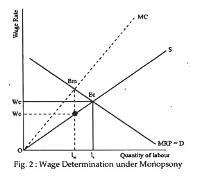
Lipsey has pointed out that, “Monopsony results in a lower level of employment and a lower wage rate than when labour is purchased com­petitively”. The reason is easy to find out: the monopsonist is aware that by trying to employ more workers, it is raising the wage rate itself. It will, therefore, stop short of the point that is reached when the factor is purchased by numerous price- taking competitive firms. This pointed is illustrated in Fig. 2.

Here, w_c and L_c are the competitive wage and employment level, respec­tively The monopsonist that must pay the same wage to all workers equates the marginal cost of hiring labour with the marginal revenue product of labour. This happens at point E_m, where the firm hired l_m workers at the wage rate w_m. The supply curve of labour here shows that at the wage rate w_m, l_m workers will be willing to work.

In the usual situation, where the labour market is characterised by a single wage monopsonist, employment and wages are less than under perfect competition. But there is an offsetting argument.

If the monopsomist can discriminate among different units of a single type of labour that it hires then two consequences will follow:

1. A discriminating monopsonist will employ more labour and make more profits than will a monopsonist who must pay the same wage to everyone.

This point is also illustrated in Fig. 2. The monopsonist does not hire more labour because doing so will drive up the wage of its existing workers. This is why its MC of hiring labour exceeds its AC. Now if the monopsonist can divide its labour into groups, it can hire a second group without pushing up the wage that has to be paid to the first group.

In this context, we may consider the extreme case in which the monopsonist can make a separate bargain with each worker, paying exactly what is necessary to persuade him (her) to accept the job. In such a situation the supply curve of labour is its MC curve and the monopsonist hires the same amount of labour as would a perfectly competitive industry.

In Fig. 2, the number of workers employed is l_c at a uniform wage of w_c and the income of workers is 0W_cE_cl_c.

A perfectly discriminating monopsonist will also hire lc of labour, but, by paying each worker his (her) supply price, the total wage bill is reduced to the area under the supply curve. This means that the area between the supply curve and the perfectly competitive wage is added to the profit of the monopsonist.

2. So, our prediction is that as long as the monopsonist can discriminate between two or more groups, employment and profits will be higher than when a single wage has to be paid.

A perfectly discriminating monopsonist can pay each worker his true supply price. In such a situation, the supply curve is also its marginal cost curve. It will employ l_c labour. Total wage income here is 0W_cE_cl_c. The triangular area 0W_cE_c is now the profit of the monopsonist (whereas under perfect competition it is part of labour’s income).