Social Welfare Economics | Environmental Economics

After reading this article you will learn about the concept of social welfare economics.

Welfare Economics studies the ways, means and methods of ensuring and increasing economic well-being of the individuals as well as the society. The subject of Welfare Economics is not merely production, exchange and consumption of goods and services; but the economic well-being or welfare. The main tool of welfare economics, therefore, is to bring the actual economy closer to ideal economy.

Satisfaction of requirements promotes welfare. In the process of satisfaction of requirements, an individual decides what is best and acts accordingly. When a person thinks what is best for him, it need not necessarily be best for the society. So, the content of term what should really govern has a social importance. It aims at the adoption of a social point of view.

In welfare economics, macro view is the only relevant view, and in this, the best way of testing a welfare proposition is to test its assumptions. There are two schools of thought regarding welfare Economics. Both schools agree that individual’s welfare is a subjective concept consisting of his utilities or satisfaction.

But, the difference is that one school regards welfare as satisfaction derived from economic goods, while the other contends that it is satisfaction derived not only from economic, but also from non-economic goods. But in practical analysis, we take only the former, keeping the latter constant.

The concept of ‘social welfare’ in welfare Economics and also its measurements are much-complicated affairs. Individual welfare is a subjective concept and we can arrive at it very easily, as.it is only additive of utilities.

Further, the scale of preference of the individual given example scope to decide the state of mind, as between two combinations and thereby arrive at comparing satisfactions. No difficulty is involved in the comparison of individual welfare; as we use the technique of individual’s choice into account.

But, on the contrary, the ‘welfare of society’ is highly elusive and an abstract term. As in the case of individual, there is no tool called ‘social choice’ to reflect unanimous social choice. So, the only way of deciding approach to define social welfare is to set down the aggregate utilities or satisfaction of all the individuals in the society.

Efficiency and Perfect Competition:

Readers will be very familiar with elementary principles of economics relating to different types of marketing conditions in the economy and how do they come to equilibrium.

In a perfectly competitive private market economy (which is rather hypothetical), the householders, otherwise called ‘consumers’ and firms, otherwise called ‘producers’ would be in large numbers and they take into account their individual welfares and decide their activities in the private competitive free market economy.

The consumers will be guided by the utilities and satisfaction they derive in demanding and consuming the goods; while the producers (firms) will be guided by the profits and losses in their ventures. In such a perfectly competitive market, no buyer or seller can affect the market price by changing the individual demand or supply in the market.

In short every operator in the market, whether consumer or supplier is only a price-taker and not price-maker. The general equilibrium price in such a market is determined by impersonal forces of market supply and demand. We assume that the level of technology, tastes, preferences and other factors remain constant without affecting the state of general equilibrium.

The left side diagram in Fig. 3.indicates the equilibrium of the perfectly competitive market arrived by the interaction of aggregate demand DD and aggregate supply SS. The firm on the right side has taken the price OP. The firm’s demand curve is the straight horizontal line at P. At the price OP, the firms can partial cost curve, which cuts the price, or revenue curve at E.

If the firm decides to produce more than OB units, it will incur loss, as MC is higher than the marginal revenue it gets for each unit sold. If it sells less than OB units, it will reap profit. But maximization of profit comes at the level OB where MC is equal to MR.

In a perfectly competitive market, a firm will maximize its profit at a level of out-put where P = MC. Every firm will produce where P = MC. Here the sellers group gets maximum benefit by making P – MC. The total market SS is equal to total market demand and in this since all consumers are satisfied as they get the quantity what they demand.

Perfect Competition and Externalities:

The goal of profit maximization leads perfectly competitive firms in equilibrium to produce at a level of output at which price equals marginal cost.

This equality between price and marginal cost is a crucial link in the chain of logic that concludes with the identification of maximum social Welfare with the outcome of a system of competitive private markets. We are now interested in examining the validity of this result once externalities are introduced.

In most context, the marginal cost schedule of a firm represents all the additions costs incurred to produce a given unit of output. The implicit assumption is that all given costs are born by the firm and thus may be termed private costs.

Given this assumption, then in the Fig. 4. the incremental costs of production could be shown as the marginal private cost (MPC) schedule. Profit maximizing behavior by the firm then yields the socially optimal output of Oe units. The MPC schedule includes the incremental costs of labour, materials and capital to the firm.

If these are the only variable costs of production, then MPC is identical to the full marginal costs of production for the whole economy. However, by emphasizing the word private in the firm’s marginal cost schedule, we do intend the possibility that other costs of production may exist.

If we use the diagram to represent the textile producers in our example, we know that the MPC understates the full variable costs of textile production. The net income loss of the farmer is an additional cost from the standpoint of the whole society, but this cost is not included in the MPC schedule of the textile firm.

Thus, we can conceive of another marginal cost schedule that includes all the costs of textile production, both private and external. We shall call this alternative the marginal social cost (MSC) schedule. As drawn in the diagram, in accordance with the assumption of our simple example, it lies above the MPC schedules at every quantity.

The vertical difference between the MPC and the MSC schedules at any given quantity measures the external (that is the fanner’s net income loss) per extra unit of output of textile production. For e.g., the MPC of producing the of^th unit of textile is P₂, but the MSC of this unit is P₁.

The difference, is marginal external cost of producing the Of^th unit of textiles. As the two schedules are drawn in the diagram the marginal external cost of the textile production is constant per unit of output and does not depends on the level of output (Geometrically, the vertical distance between the MSC and MPC schedules is same at all levels of output).

As we are assuming that all markers are perfectly competitive, we know that the textile produce cannot affect the running market price shown in the Fig. 4. as the horizontal line P_T. Because the manager of the textile firm takes into account only the firm’s private cost, he maximizes profits by production of an output of Oe units, where P_T = MPC.

From society’s standpoint, however, all costs-private and external should be accounted for in determining optimal levels of output. Ideally, the price-marginal cost equality should occur at the output. Ideally the price marginal cost equality should occur at the output levels where P_T = MSC. or On in diagram.

This reasoning allows us to conclude that the excess of (Ne) units between the private optimal level of production (Oe) and the social optimal level (On) represents overproduction of textiles.

Society would be better off with (On) units of textile production than with (Oe) units because resources used to produce the last (Ne) units have greater net productive value in other employment. The same reasoning implies of course, that some other good or goods in the economy are being under produced or not produced at all.

Thus the first result of our analysis is simply that an external diseconomy, in otherwise ideal competitive market system distorts the optimal allocation of resources; the quantities produced of some goods are too large and this implies that the quantities produced of other goods are too small.

The aggregate of all textile firms with similar marginal cost conditions can be summarized in the industry. Supply of each textile firm is its supply schedule. The MPC schedule of each textile firm is its supply schedule at all price levels that exceed average variable costs.

The textile industry supply schedule is simply the horizontal summation of the MPC schedules of all the individual textile firms e.g., if each firm produces Oe units at a price of P_T as in the diagram Fig. 5. Then n-identical firms will produce at this price on units of output for the entire industry.

Any point on the industry supply can be obtained conceptually by adding the quantities that each firm would offer for sale at the relevant price. Such a supply schedule is drawn for the textile industry as its (private) supply schedule. PSS in the Fig. 5.

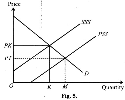
A similar summation of the MSC schedule of all textile firms is also shown in the diagram Fig. and is labelled SS for social supply schedule. The SS curve lie above the PS curve, reflecting the difference between marginal private cost and social cost for all firms in the industry which, schedules at any point is the aggregate of the external costs, imposed on society for a given level of output by the industry.

According to our previous assumptions the SS schedule, not the PS schedule, reflects the social marginal costs of textile output. Embodied in the SS schedule is the value of the foregone predication and all the other external costs imposed on firms and households in society by textile production.

If SS were the industry supply schedule in diagram the level of industry output would be OK units and the market price would be P_K Comparing this result with the actual industry price and output in equilibrium, we can conclude that the private market for textile leads to too large production of textiles (by KM = OM-OK) units and too low a price (Pi instead of P_K).

Also implicit in this conclusion is that some other industries are precluded from producing enough. Society as a whole would be better off if textile firms behaved as if SS and not PS were the industry supply schedule. At an output level of OK, they will be equal to industry output (OK) times the difference between SS and PS.

As a final observation, we may note that in the absence of any government intervention the external diseconomies of textile production lead, via the invisible hand of the profit incentive to visible pollution and but on some social costs. This conclusion holds, even under the assumption of the otherwise private market system.

Definition and Meaning of Pareto Efficiency:

“Pareto efficiency is defined as a situation in which everyone is so well off and it is impossible to make anybody better off without simultaneously making at least one person worse off. It is a situation in which all possibilities for voluntary more efficiently, have been exhausted. There are no more opportunities to improve the efficiency of the economic system.”

In a sense, Pareto efficiency is a situation so efficient that it is impossible to reallocate resources or redistribute commodities in order to make thinks more efficient. Once Pareto- efficiency has been attained, all gains to individuals must come at the expense of other individuals.

The next step in our discussion is to show that perfectly competitive Market economy with general equilibrium price discussed already, satisfies the necessary condition for maximizing social welfare. We shall limit our discussion only to P = MC result indicated in the perfectly competitive market system with the relationship of MXSW.

The society attains maximum social welfare (MXSW) when the society produces at that level of output where p = mc. How is this so? What is the relationship between MXSW and P = MC.

According to our analysis all profit maximizing firms will produce at the level of output in which the cost of last unit produced (Marginal cost or MC) will be just equal to the prevailing market price of its output. Suppose for illustration, MC is not equal to price for some reason or the other and it is greater than price (MC > P).

This means that the cost of the last unit of the commodity produced is greater than the market price of the last unit offered for sale. Evidently, the producer has to use more productive input of greater value than the price paid by the household. Price paid by household is less than of input. This in essence reveals that the economy is producing more than price what is actually required by the household.

This suggests that the production can be reduced and thereby productive input resources could be released for using the same for more socially valuable commodity. This type of cost – benefit tests determine the optimum levels of production in the economy.

Further, in such a situation where MC not equals to P the profit maximization behavior of the firm will be upset. Thus we come to the conclusion that MC = P is a necessary condition for MXSW in a perfectly competitive system, and the market becomes more efficient with allocation of resources.

Maximum Social Welfare and Perfect Competition:

(Analysis with Indifference Curves)

Indifference Curve technique can be used for analyzing the concept of maximum social welfare with available resources to indicate that perfect competition is a necessary condition for achieving Pareto’s efficiency of Optimum Welfare.

We can start with household equilibrium in consumption with IC technique, as indicated in the diagram Fig. 6. In the diagram, WC₁, WC₂, WC₃ etc., indicate levels of welfare (satisfaction in consumption of two commodities of the i.e., household X and Y) with given quantum resources for the household.

The assumption is that the households behave rationally and attempt to maximize their economic welfare by selecting the largest and best collection of goods X and 7 with its resources.

Further, we assume perfect competition in the market, and prices of X and Y remain constant. Higher WC indicates higher levels of satisfaction, i.e., welfare. The consumption possibility line with given prices of X and Y is AB watch is called the budget line of the household.

The household can allocate the resource in any way it likes by; moving on the budget line AB, selecting X and Y commodities. The convex nature of the indifference curves indicates that the significance of X commodity; diminishes, as it chooses more of X rejecting some of Y commodity and vice versa.

The marginal rate of substitution between X and Y commodities diminishes, as the household chooses to travel down on the WC. In difference curve analysis, the slope of the budget line or the price line represents the ratio of the prices of two commodities, i.e., X and Y.

OA/OB = Px/Py

Further, at the point E, the slope of budget line AB and the slope of WC₂ are the same. We have studied under ‘indifference curve’ analysis that the slope of the indifference curve represents the marginal rate of substitution of X and K commodities and the slope of the price, line i.e., budget line indicates the ratio of price of two goods. Hence, at equilibrium point, the marginal rate of substitution between two goods is equal to the ratio of their price.

That is at equilibrium MRSxy = Px/Py

In the same way, in this analysis, we take the optimal point E on the WC₂ (welfare curve) where the slope of the welfare curve is equal to the slope of the budget line. To restate, we can say: Price of X commodity/Price of Y commodity = Marginal welfare of X/Marginal welfare of Y.

The logic of this conclusion can be well understood as follows:

Suppose, any household does not consume any pair of goods so as to attain this maximum condition, it can increase its welfare by shifting some of its expenditures from the commodity with a relatively low MfV/P to one with higher MW/P. In our illustration, moving from E₁ to E along line AB. At point E₁, MWx/Px will be smaller than MWx/ Py.

By substituting Y commodity in the place of A’ commodity, which can be done by moving up on the budget line, the household can reach the higher we If; ‘e curve, i.e., from WC₁ to WC₂ .This will be possible only under the assumption of perfect competition in which the price ratio Px/Py is a constant parameter for any household.

Further, this has an important significance for the interpretation of relative prices in a perfectly competitive economy in a state of general equilibrium. All relative prices such as Px/Py = MWx/Mwy measure exactly for every household the relative subjective contribution of economic welfare of the last units of goods and services consumed.

The price of every commodity measures the benefit of the last unit consumed, i.e., marginal welfare for any household in the economy is equilibrium. In the aggregate, this will be the outcome of individual household cost-benefit decisions of all types made by millions of households.

Firm’s Equilibrium in Production:

The above analysis will help to show that only in a perfectly competitive economy, the firm can maximize profit to maximize welfare. We had already discussed that in a perfectly competitive market, the firm will produce at a level where P = MC.

This means that every firm in the economy produces its output to a point where price is equal to marginal cost. The price of X is the marginal cost of X. This means Px = MCx. In the same way Py = MCy. It follows that relative prices will be exactly equal to relative marginal costs for all products and services, i.e., Px/Py = MCxMCy.

This connotes that relative price of all goods measures the relative marginal costs of all goods in a perfectly competitive economy in equilibrium. All these go to show that there will be maximum efficiency in a perfectly competitive economy in equilibrium, and all the people will attain maximum satisfaction and Pareto’s maximum social welfare could be obtained.

Consideration of Externality in a Monopolistic Firm:

Now, we have come across two sets of problems distorting the efficiency of the market. The first one relating to prefect competition in which the external costs cause price to fall below the true marginal social cost of production and the resulting level of output is too high compared to the level where all costs are paid by the firm.

That is, under perfect competition, the firms produce more at a lesser price. On the other hand, in the case of monopoly, the firm produces less and prices at a higher level, i.e., more than the marginal cost.

These two effects work in opposite directions and will tend to offset each other. Any one of these two effects may dominate. It will be very difficult to determine theoretically which effect is stronger, as it is an empirical problem.

Next, we shall take up the consideration of externality in a monopolistic firm. Suppose, the monopoly firm generates pollution and imposes external costs on the society. Based on maximizing behavior without considering the externality, the monopolist will produce OM units selling at a price OPm as shown in the diagram Fig. 7.

The marginal cost curve will become the marginal private cost (MPC) and the marginal social cost curve (MSC) will lie above MPC at a distance of pollution cost for every unit produced. The equilibrium point ‘F’ which is socially advantageous is shown in the diagram.

When the firm internalizes the external cost, the level of output will be OL and the price will be OP_L as shown in the diagram. Now the situation presents two distortions; the existence of monopoly and the existence of external cost.

Correction of both problems is necessary to obtain the socially efficient outcome. Economists call such a situation, the problem of Second Best. If only one of these two distortions alone is set right, the society will not necessarily be better off. In terms of efficiency, the situation remains unchanged.

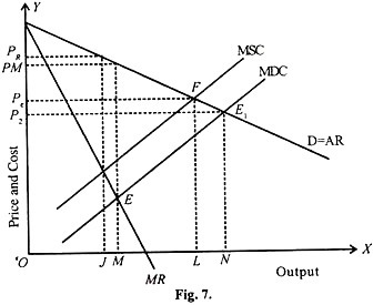
Suppose by starting a tirade either socially, politically or legally against the monopoly firm and the situation is brought to the level of perfect competition without internalizing the external cost, then the output will expand to the level of ON and the price will fall to OP_n.

This correction is rather unwarranted, as the output will expand far beyond the socially optimum level. Whether output OM is more efficient or output ON is more efficient relative to the socially optimum level of output OL is rather very difficult to judge by theory, as it becomes an empirical study. It is better to leave the monopoly alone which will be more efficient, than bringing about a situation of competition.

Suppose in our illustration the government imposes a tax on the monopolist to curb his production activities to neutralize the pollution or external cost. The amount of the tax per unit of production cannot be more than the external cost of pollution per unit.

In that case, the monopolist will behave as if the MSC is his MPC, as tax paid will be brought into cost of production. The monopolist will find his equilibrium by equating marginal social cost will marginal revenue and reduce the output to the level of OJ at a price Pj as shown in the diagram.

This situation is far worse than the original monopolistic equilibrium. By the imposition of the tax, the level of production has decreased very much from the socially optimum level of OL with a conspicuous increase in price (P), which is higher than the monopoly price OP_m.

This level of output is decidedly less efficient socially than the output of OM level, since this level is far less than the socially optimum level of OL. From this, it is evident that it would be better from society’s point of view not to impose a tax to internalize the external costs.

Thus, we infer, when an industry is characterized by monopoly as well as externality, better result will not come out by treating them individually and piecemeal. Both problems have to be jointly treated to achieve better resource allocation efficiency. If we attempt to correct only one deficiency of the two deficiencies, namely monopoly and externality, the result will be loss of social welfare. The remedy will be worse than the malady.

The cumulative effect of monopoly with externalities cannot be determined without empirical examination, case by case, to assess the extent of each problem. The environmental policy and anti-trust activities should be well coordinated to find solution for the cases.