Controlling Pollution and Externalities | Environmental Economics

This article throws light upon the top two measures used to control pollution and externalities. The measures are: 1. Imposing a Pigouvian Tax 2. Environmental Regulation.

Measure # Imposing a Pigouvian Tax:

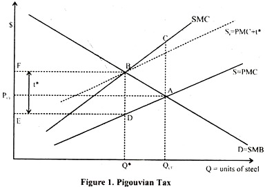
A “classical” representation to the externality problem, due to Pigou (1920), is depicted in Figure 1. The horizontal axis denotes output of a competitive industry, say steel, which generates a negative externality, say smoke and dust that harms nearby homeowners.

D is the demand curve which (as you should know from Micro) reflects the marginal social benefit of producing steel. S is the industry supply, or, more relevant for our purposes, the private marginal costs of producing steel (the costs of coal, ore, labour etc.) There is additional cost of producing steel – the harm to homeowners.

The picture assumes that the total as well as marginal harm is increasing in steel output. The social marginal costs of producing steel (curve SMC) are the sum of private marginal costs to producers and the marginal harm to homeowners.

The competitive equilibrium occurs where the private marginal costs are equal to marginal benefit, so the Competitive price will be PCE and the competitive output QCE. The socially optimal level of output would, however, equate the social marginal costs with marginal benefit, which happens at Q*. More than the efficient amount of steel is produced, and the deadweight costs of the externality is the triangle ABC.

Pigou’s solution was to impose a tax on each unit of output. The industry would face higher private marginal costs (the costs of input plus the tax) and the competitive output would be reduced. The optimal tax replicates the efficient outcome.

The Figure 1 shows that the optimal tax t* is equal to the difference between social and private marginal costs at the efficient level of output (the length of abscissa BD). The industry supply curve shifts up to St and it intersects the demand curve exactly at output Q*. The government collects tax revenue equal to the area BDEF.

There are a few problems with this approach:

(1) It tacitly assumes a given technology translating output into pollution. Reduction in pollution occurs only through reduction in output rather than through an implementation of different technology (scrubbers) that reduces pollution at a given level of output.

(2) If producers differ in pollution technology (some pollute less than others at the same level of output) the tax is inefficient. For low-pollution producers, it exceeds the marginal harm that they cause, thus inducing them to cut output too much, and vice versa for high-pollution producers.

You can see that these two points boil down to the fact that the tax does not deal with the pollution directly, but only through output. A straightforward way out is to levy the tax on pollution – say to charge $10 for each tonne of smoke particles emitted (at important requirement here is that we can measure the pollution).

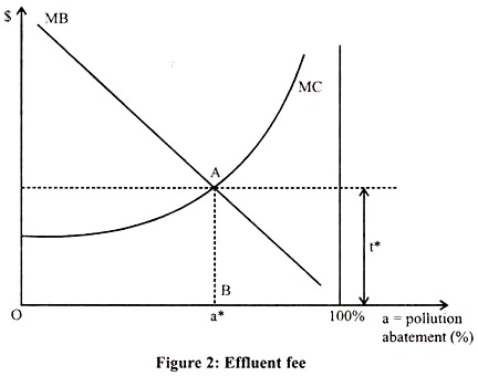
The tax on pollution is sometimes called an effluent fee and is depicted in Figure 2. The horizontal axis denotes a reduction in pollution (or pollution abatement, a) in per cent.

The origin is associated with the level of pollution at the time before any effluent fee or some other policy is implemented; 100% abatement means that no smoke is emitted. The marginal cost of pollution abatement is increasing in a. Note this is a cost function – the least cost way for the firm of abating pollution by one unit, which could be achieved by cutting output or installing some pollution reduction technology.

The socially optimal level of abatement equates the marginal costs of abatement with marginal benefit point a*. The optimal abatement can be implemented by an effluent fee t* equal to the marginal benefit of abatement at a*.

For the firm, the marginal benefit of reducing pollution by one unit, is t: this is what the firm saves on tax liability if it cuts pollution by one unit. For a < a*, the tax is greater than the marginal cost, so it is profitable for the firm to increase pollution abatement up to the point where the tax is equal to marginal cost: i.e., up to a.

The problem can be easily expressed in mathematical terms: Let function B (a) represent the total benefits of pollution abatement, which is increasing and concave in a. The total cost of abatement, C (a) is increasing and convex, and C (1) = (it is prohibitively expensive to achieve a complete cleanliness).

The social planner’s problem is to maximize the benefit net of cost:

Max B(a)-C(a)

a

The optimum is characterized by the first-order condition:

B'(a) = C'(a)

which means that marginal benefit is equal to marginal cost. Note that the efficient level of pollution abatement is not 100%. Now if the polluter faces an effluent fee t per unit of pollution, he wants to minimize his total cost of pollution, which include the fee plus the costs of reducing the fee. Hence the firm’s problem is:

min C(a) + (1 a)t

The optimal level of abatement for the firm is given by

C'(a) = t

It is straightforward to see that if we set t = B'(a), the optimal level of a for the firm is identical to the socially optimal level.

Measure # Environmental Regulation:

An alternative to Pigouvian taxes is regulation. The government tells polluters how much they have to cut pollution, and often times it even says what particular technology they have to use to cut pollution. Finns do not do any private optimization under regulation – they simply do what the government tells them to do.

In principle, regulation can perfectly replicate the outcome of the effluent fee – the government tells firms to cut pollution to a*, and that is efficient. There are, however, important differences when it comes to implementation

Note than by the effluent fee, the government directly affects only the total level of pollution. If it thinks there should be less pollution, it can increase the tax, and vice versa. The distribution of pollution is left to market forces: each polluter will make his own calculation as to how much it pays to invest in pollution abatement.

All polluters will cut pollution up to the point when their marginal costs of cutting pollution are equal to the tax per unit. This implies that any level of total pollution abatement in achieved at minimum cost, (can you see why?) The government needs to know only the marginal benefits of pollution abatement, not the technology.

Under regulation, the government sets not only the total level of abatement, but also the level for each polluter. For such a policy to be optimal, the government has to know everything – the social benefits of abatement, the costs of abatement for each polluter, the technologies available.

Thus efficient regulation has much larger informational requirements than an efficient effluent fee. For this reason, regulation is by its nature bound to be less efficient than the effluent fee: Regulation can always replicate the same total abatement as the fee but While the distribution of abatement across pollution sources is always efficient under the fee, it is efficient under regulation only has perfect information, and that we know is impossible.

Despite the theoretical appeal, Pigouvian taxes are used rarely (a big exception is the gasoline tax, although that’s a tax on input), while regulation prevails. The actual regulation as carried out in the USA by the Environmental Protection Agency (EPA) is very centralized and heavy-handed.

Aside from setting broader goals and standards, EPA can (and often does) say what should be done with a particular pollution source. Two general features of the EPA policy are worth mentioning here: One is the tendency to make the regulations stricter for new sources of pollution than for existing sources.

Second is the tendency to make the standards universal – same levels of pollution or percentage abatements are required from all existing sources, regardless of how the costs of abatement differ among them, or where they are located (the benefits of cutting pollution are generally higher for sources located in populated areas). To demonstrate, here is a quote from a randomly selected recent EPA regulation regarding copper smelters:

“1. Copper Concentrate Dryers: The proposed standards establish emission limits for particulate matter contained in the exhaust gases discharged from each affected copper concentrate dryer. Separate emission standards would be established for existing sources and new sources. The standard would limit the concentration of particulate matter discharged from existing copper concentrate dryers to no more than 50 milligrams per dry standard cubic meter (mg/dscm) (approximately 0.022 grains per dry standard cubic foot (gr/dscf). New copper concentrate dryers would be limited to no more than 23 mg/dscm (approximately 0.01 gr/dscf) of particulate matter. The rule would allow an owner or operator to use any type of particulate control device (i.e., bag-house, electrostatic precipitator, or wet scrubber) that meets the applicable PM emission limit.”

Don’t worry even if you do not understand the technical content, you may see that different rules apply to new and old sources, but within each group, the level of emissions has to be same for each source.

The problem with uniform standards is that as the costs and benefits of pollution abatement differ among sources, the optimal level of abatement is different for each source, and therefore uniform standards do not implement the efficient solution.

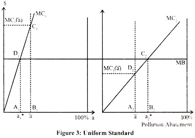
The consequences of uniform standards are shown in Figure 3. Again, the level of pollution abatement is on the horizontal axis, and the marginal benefit is for simplicity assumed to be constant. There are two polluters, firms 1 and 2.

They have different marginal costs of pollution abatement – firm 1 is the high-cost firm, since for every level of abatement, MCI (a) > MC2 (a). Efficiency requires that the marginal costs of abatement are equal to the marginal benefit for each firm:

MC₁(a*1) = MC2(a*2) = MB

where a and a* denote the socially efficient abatement for each firm. Notice that the marginal costs are equalized across both sources. Finn 1 reduces pollution by a smaller amount than firm 2 (a*l< a*2), since it is more costly for the firm 1 to reduce pollution.

Let us now consider a regulation that achieves the same total reduction in pollution by uniform standard – each firm has to abate pollution by the same amount a, and a = (a*l + a*2)/2. You can see that the marginal costs of pollution are not equalized across firms: MCI (a) > MC2 (a). Why is this inefficient?

Keep in mind that the total level of pollution abatement is the same under the optimal tax and the uniform standard, so we can set the benefits aside and focus only on the costs. Finn 1 has to reduce pollution more, so what is the cost to firm 1 of moving from a*l to a? It is the area of the trapezoid A1B1C1D1.

Firm 2 makes a smaller reduction in pollution, so how much does it save by moving from a*2 to at a? It saves the area of the trapezoid A2B2C2D2.Since a*l-a = a*2 – a by construction of the average, it is straightforward to compare the trapezoids and see that the cost to firm 1 exceeds the savings to firm 2. Hence the uniform standard achieved the same reduction in pollution at higher cost.

This problem with uniform standards has been recognized since the beginning and many studies attempted to measure its magnitude. The first such study was Kneese and Bower (1968).

They went down all the pollution sources along the Delaware River and estimated the cost function of pollution abatement for each source. From that, they computed the total cost of abatement under the actual EPA policy and compared them with the costs of achieving the same level of pollution by optimal allocation across sources.

They found that the EPA policy was twice as costly as the minimum-cost solution. Numerous similar studies of different types of pollution in different places produced a range of estimates ranging from 1.1 to 22. On average, EPA regulations were found to achieve the reduction in pollution at about 4 to 6 times higher costs than necessary.

Another solution to the externality problem had existed long before economists started thinking about environmental regulations and Pigouvian taxes. Common law has traditionally allowed the persons whose property or health were negatively affected by actions of other persons to sue them.

The remedies offered by the courts were either damages (the pollute has to compensate the victim of pollution) or injection (the court orders the polluter to stop the harm; in legal parlance, the court enjoins the polluter).

We will spend a good deal of time studying both remedies; at this point observe that the damages remedy looks very much like the effluent fee: the polluter has to pay for all the harm that he is causing, if he pollutes less, he will pay less, so he bears all the costs of pollution – we say that he internalizes the externality.

The polluter compares the damages with the costs of reducing the harm and decides whether and how much it pays to reduce the harm. Since he bears all the costs, he will set the level of pollution at the efficient level. The big difference between the damages and the fee is that the damages go to the victim of pollution, while the fee goes to the government.

The traditional view of legal liability was that if the polluter has to pay damages, he will reduce pollution to the efficient level, while if he does not have to pay damages (the court says he is free to pollute), he will not cut pollution at all.

Seems obvious, does not it? Actually, Ronald Coase showed that it is not true, and that no matter what the legal rule is, the pollution will always be set to the efficient level (under certain conditions).