Neoclassical Theory of Economic Growth | India | Economics

In this article we will discuss about:- 1. Introduction to the Neoclassical Theory of Economic Growth 2. Production Function and Saving of Neoclassical Growth Theory 3. Fundamental Growth Equation of Neoclassical Growth Theory 4. The Growth Process 5. Impact of Increase in the Saving Rate 6. Effect of Increase in Population Growth Rate 7. Long-Run Growth and Technological Change.

Introduction to the Neoclassical Theory of Economic Growth:

The neoclassical growth theory was developed in the late 1950s and 1960s of the twentieth century as a result of intensive research in the field of growth economics. The American economist, Robert Solow, who won a Nobel Prize in Economics and the British economist, J. E. Meade, are the two well-known contributors to the neoclassical theory of growth. This neoclassical growth theory lays stress on capital accumulation and its related decision of saving as an important determinant of economic growth. Neoclassical growth model considered two factor production functions with capital and labour as determinants of output. Besides, it added exogenously determined factor, technology, to the production function. Thus neoclassical growth model uses the following production function–

Y= AF (K, L) … (1)

Where, Y is Gross Domestic Product (GDP), K is the stock of capital, L is the amount of unskilled labour and A is exogenously determined level of technology. Note that change in this exogenous variable, technology, will cause a shift in the production function.

There are two ways in which technology parameter A is incorporated in the production function. One popular way of incorporating the technology parameter in the production function is to assume that technology is labour augmenting and accordingly the production function is written as–

Y= F (K, AL) … (2)

Note that labour-augmenting technological change implies that it increases productivity of labour. The second important way of incorporating the technology factor in the production function is to assume that technological progress augments all factors (both capital and labour in our production function) and not just augmenting labour. It is in this way that we have written the production function equation (1) above.

To repeat, in this neoclassical approach production function is written as-

Y=AF (K, L)

Considering in this way, A represents total factor productivity (that is, productivity of both factor inputs). When we empirically estimate production function specified in this way, then contribution of A to the growth in total output is called Solow residual which means that total factor productivity really measures the increase in output which is not accounted for by changes in factors, capital and labour.

Unlike the fixed proportion production function of Harrod-Domar model of economic growth, neoclassical growth model uses variable proportion production function, that is, it considers unlimited possibilities of substitution between capital and labour in the production process. That is why it is called neoclassical growth model as the earlier neoclassical considered such a variable proportion production function. The second important departure made by neoclassical growth theory from Harrod- Domar growth model is that it assumes that planned investment and saving are always equal because of immediate adjustments in prices (including interest). With these assumptions, neoclassical growth theory focuses its attention on supply-side factors such as capital and technology for determining rate of economic growth of a country.

Therefore, unlike Harrod-Domar growth model, it does not consider aggregate demand for goods limiting economic growth. Therefore, it is called ‘classical’ along with ‘neo’. The growth of output in this model is achieved at least in the short run through higher rate of saving and therefore higher rate of capital formation. However, diminishing returns to capital limit economic growth in this model. Though the neoclassical growth model assumes constant returns to scale which exhibits diminishing returns to capital and labour separately.

Below, neoclassical growth model explains economic growth through capital accumulation (i.e., saving and investment) and how this growth process ends in steady state equilibrium. By steady state equilibrium for the economy we mean that growth rate of output equals growth rate of labour force and growth rate of capital (i.e., ∆Y/Y =∆L/L=∆K/K) so that per capita income and per capita capital are no longer changing. Note that income per capita and capital per worker to remain constant in this steady state equilibrium when labour force is growing implies that income and capital must be growing at the same rate as labour force. Since growth in labour force (or population) is generally denoted by letter ‘n’, in this steady state equilibrium, therefore, ∆Y/Y=∆K/K= ∆N/N=n Neoclassical growth theory explains the process of growth from any initial position to this steady state equilibrium.

Production Function and Saving of Neoclassical Growth Theory:

As stated above, neoclassical growth theory uses following production function–

Y = AF (K, L) …(1)

However, the neoclassical theory explains the growth process using the above production function in its intensive form, that is, in per capita terms. To obtain the above production function in per capita terms we divide both sides of the given production function by L, the number of labour force. Thus–

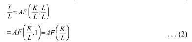
To begin with we assume that there is no technological progress. With this assumption then equation (2) is reduced to-

Y/L=F (K/L) …..(3)

The equation (3) states that output per head (Y/L) is a function of capital per head (K/L). Writing y for Y/L and k for K/L equation (3) can be written as-

y=f(K) ……(4)

Now, in Fig. 14.1 we represent the production function (4) in per capita terms. It will be noticed from Fig. 14.1 that as capital per capita (k) increases, output per head increases, that is, marginal product of labour is positive. But, as will be seen from Fig. 14.1, the slope of the production function curve decreases as capital per head increases. This implies that marginal product of capital diminishes. That is, the increase in capital per head causes output per head to increase but at a diminishing rate.

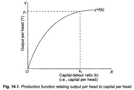
It will be seen from Fig. 14.1 that at capital-labour ratio (i.e., capital per worker) equal to k_1, output per head is y₁ . Similarly, we can read from the production function curve y = f (k) the output per head corresponding to any other capital per head.

Fundamental Growth Equation of Neoclassical Growth Theory:

According to neoclassical theory, rate of saving plays an important role in the growth process of an economy. Like the Harrod-Domar model, neoclassical theory considers saving as a constant fraction of income. Thus–

S = sY …(5)

Where, S = saving

Y= income.

s = propensity to save

Since s is a constant fraction of income, average propensity to save is equal to marginal propen­sity to save. Further, since national income equals national product, we can also write equation (5) as

sY = sF(K, L)

As in neoclassical theory, planned investment is always equal to planned saving, net addition to the stock of capital is ∆K, which is the same thing as investment (I), can be obtained by deducting depreciation of capital stock during a period from the planned saving. Thus–

∆K = I = sY-D …… (6)

Where, ∆K = net addition to the stock of capital, I stands for investment and D for depreciation. Depreciation occurs at a certain percentage of the existing capital stock. The total depreciation (D) can be written as–

D = dK

Substituting dK for D in equation (6) we have

∆K = sY – dK

Or sY = ∆K + dK…… (7)

Now dividing and multiplying the first term of the left-hand side of equation (7) by K we have–

sY = K.(∆K/K) + dK ……. (8)

We have seen above that for the steady state equilibrium, growth of capital (∆K/K) must be equal to growth of labour force (∆L/L), so that capital per worker and therefore income per head remains constant. If we denote growth rate of labour force (∆L/L) by n, then in steady state ∆K/K = n. Substituting n for ∆K/K in equation (8) we have–

sY = K . n + dK

or sY=(n + d)K …(9)

The above equation (9) is a fundamental growth equation of the neoclassical growth model and states the condition for the steady-state equilibrium growth rate when capital per worker and therefore income per capita remains constant even though population or labour force is growing. Thus, for steady-state growth equilibrium capital must be increasing equal to (n + d) K. Therefore (n + d) K represents the required investment (or change in capital stock) which ensures steady state when capital and income must be growing at the same rate as labour force (or population).

The Growth Process of Neoclassical Growth Theory:

From the growth equation (9) it is evident that if planned saving sY is greater than the required investment (i.e., (n + d) K) to keep per capita income constant, capital for worker will increase. This increase in capital per worker will cause increase in productivity of worker. As a result, the economy will grow at higher rate than the steady-state equilibrium growth rate. However, this higher growth rate will not occur endlessly because diminishing returns to capital will bring it down to the steady rate of growth, though at a higher level of per capita income and capital per worker.

In order to graphically show the growth process, the growth equation is conventionally used in intensive form, that is, in per capita terms. In order to do so we divide both sides of equation (9) by L and have –

sY/L=(n=d)K/L

Where, Y/L represents income per capita and K/L represents capital per worker (i.e. capital-labour ratio).

Writing y for Y/L and k for K/L we have

sy = (n + d)k …(10)

The equation (10) represents fundamental neoclassical growth equation in per capita terms.

Growth Process and Steady Growth Rate:

Fig. 14.2 shows the growth process that moves the economy over time from an initial position to the steady-state equilibrium growth rate. In this Fig. 14.2 along with per capita production function (y =f(k)) we have also drawn per capita saving function curve sy. Besides, we have drawn (n + d)k curve which depicts required investment per worker to keep constant the level of capital per capita when population or labour force is growing at a given rate n.

In Fig. 14.2, y =f(k) is per capita production function curve as in Fig. 14.1. Since per capita saving is a constant fraction of per capita output (i.e. income), the curve sy depicting per capita saving function is drawn below the per capita production function curve (y =f(k)) with the same shape.

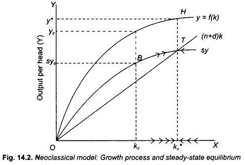
Another straight line curve labeled as (n+d)K, is drawn which depicts the required investment to Keep capital per head (i.e., capital –labour ratio) constant at various levels of capital per head .

Now, let us assume the current capital per head is k₀ at which per capita income (or output) is y₀ and per capita saving is sy₀. It will be seen from Fig. 14.2 that at capital per head k₀, per capita saving sy exceeds investment required to maintain capital per head equal to k₀ (sy₀ > (n + d)k). As a result, capital per head (k) will rise (as indicated by horizontal arrows) which will lead to increase in per capita income and the economy moves to the right. This adjustment process will continue so long as sy > (n + d) k. It will be seen that when the economy reaches at capital per head equal to k* and per capita income equal to y* corresponding to which saving curve sy interests the (n + d) k curve at point T.

It will be noticed from Fig. 14.2 that the adjustment process comes to rest at capital per head equal to k* because saving and investment corresponding to this state is equal to the investment required to maintain capital per head at k*. Thus point T and its associated capital per head equal to k* and income or output per head equal to y* represent the steady-state equilibrium. It is worth noting that whether the economy is initially at the left or right of k*, the adjustment process leads to the steady state at point T. It may however be noted that in steady-state equilibrium, the economy is growing at the same rate as labour force (that is, equal to n or ∆L/L).

It will be seen from Fig. 14.2 that although growth of economy comes down to the steady growth rate, its levels of per capita capital and per capita income at point T are greater as compared to the initial state at point B.

An important economic implication of the above growth process visualised in neoclassical growth model is that different countries having same saving rate and population growth rate and access to the same technology will ultimately converge to same per capita income although this convergence process may take different time in different countries.

Impact of Increase in the Saving Rate:

In the steady state, both capital per head (k) and income per head (y) remain constant when economy is growing at the rate of growth of population or labour force (i.e., n). In other words, in steady-state equilibrium ∆k = 0 and ∆Y = 0.

It follows from this that steady-state growth rate or long-run growth rate which is equal to population or labour force growth rate n is not affected by changes in the saving rate. Changes in the saving rat affect only the short- run growth rate of the economy. This is an important implication of neoclassical growth model.

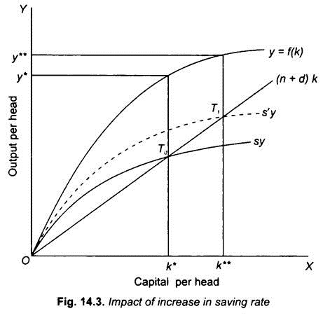
Now an important question is why do we get this apparently incredible result from the neoclassical growth theory? Impact of increase in the saving rate is illustrated in Fig. 14.3. It will be seen from this figure that initially with the saving curve sy, the economy is in steady state at point T₀ where the saving curve sy intersects required investment curve (n + d) k with k* as capital per head and y* as income (output) per capita. Now suppose that saving rate increases, that is, individuals in the society decide to save a higher fraction of their income. As a result, saving curve shifts to the new higher position s’y (dotted). This higher saving curve s’y intersects the (n + d) k curve at point T₁ which therefore represents the new steady state.

We thus see that increase in saving rate moves the steady-state equilibrium to the right and causes both capital per head and income per head to rise to k** and y** respectively Note that in the new steady state the economy grows at the same rate as the growth rate of labour force (or population) which is denoted by n. It therefore follows that long-run growth rate of the economy remains unaffected by the increase in the saving rate though the steady state position has moved to the right.

Two points are worth noting here. First, though long-run growth rate of the economy remains the same as a result of increase in the saving rate, capital per head (k) and income per capita (y) have risen with the upward shift in the saving curve to s’y and consequently the change in steady state from T₀ to T₁, capital per head has increased from k* to k** and income per head has risen from y* to y**.

However, it is important to note that in the transition period or in the short run when the adjustment process is taking place from an initial steady state to a new steady state, a higher growth rate in per capita income is achieved. Thus, in Fig. 14.3 when with the initial steady state point T₀, saving rate increases and saving curve shifts upward from sy to s’y, at the initial point T₀, planned saving or investment exceeds (n + d) k which causes capital per head to rise in the short run resulting in a higher growth in per capita income than the growth rate in labour force (n) till the new steady state is reached.

The effect of increase in saving rate on growth of output or income per head (y) and growth rate of total output(i.e., ∆Y/Y) is shown in Fig. 14.4 (a) and 14.4 (b). Fig. 14.4 (a) shows the growth in output (income) per head as a result of increase in the saving rate. To begin with, the economy is initially in steady-state equilibrium at time t₀ with output per head equal to y*. The increase in saving rate causes capital per head to rise which leads to the growth in output per head till time is reached. At time t₁ the economy is again in steady-state equilibrium but now at a higher level y** of output per head. Note that in the transition pursued from to t₀ to t₁ output per head increases but at a diminishing rate.

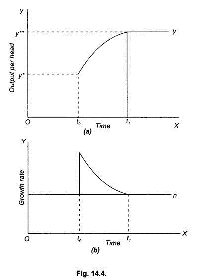
Fig 14.4 (b) Illustrates the adjustment in the growth rate of total output (i.e ∆Y/Y).It will be seen from Fig. 14.4 (b) that starting from initial steady state at time t₀ the increase in saving rate and capital formation leads to growth rate in total output higher than the steady growth rate n in the period from t₀ to t₁ but in period t₁, it returns to the steady growth rate path n. It is thus evident that the higher saving rate leads to a higher growth rate in the short run only, while long-run growth rate in output remains unaffected.

The increase in the saving rate raises the growth rate of output in the short run due to faster growth in capital and therefore in output. As more capital is accumulated, the growth rate decreases due to the diminishing returns to capital and eventually falls back to the population or labour force growth rate (n).

Effect of Increase in Population Growth Rate:

For developing countries like India it is important to discuss the effect of increase in population growth rate on steady levels of capital per head (k) and output per head (y) and also on the steady- state rate of growth of aggregate output. Fig. 14.5 illustrates these effects of increase in population growth. An increase in population growth rate causes an upward shift in (n + d) k line. Thus in Fig. 14.5, the increase in population growth rate from n to n’ causes upward shifts of (n + d) k to (n’ + d) k curve (dotted). It will be seen from Fig. 14.5 that the new (n’ + d) k curve cuts the given saving curve sy at point T’ at which capital per head has decreased from k*₁ to k*₂ and output per capita has fallen from y*₁ to y*₂.

This can be easily explained. Due to higher growth rate of population a given stock of capital is spread thinly over labour force which results in lower capital per head (i.e., capital-labour ratio). Decrease in capital per head causes decline in per capita output. This is an important result of neoclassical growth theory which shows that population growth in developing countries like India impedes growth in per capita income and therefore multiplies our efforts to raise living standards of the people.

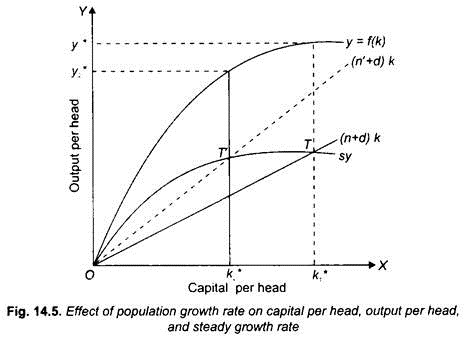
Fig. 14.5 also shows that higher growth rate of population raises the steady-state growth rate. It will be seen from this figure that increase in population growth rate from n to n’ causes (n + d) k curve to shift upward to the new position (n’ +d) k (dotted) which intersects the saving curve at new steady-state equilibrium point T’. The steady-state growth rate has therefore risen to n’, that is, equal to the new growth rate of population. It may however be noted that higher steady rate of growth is not a desirable thing.

As a matter of fact, a higher steady growth means that to maintain a certain given capital-labour ratio and per capita income the economy has to save and invest more. This implies that a higher rate of population acts as an obstacle to raise per capita income and therefore living standards of the people. Thus, this result provides a significant lesson for the developing countries like India, that is, if they want to achieve higher living standards for its people they should make efforts to control population growth rate.

Long-Run Growth and Technological Change:

Let us now analyze the effect of technological change on long-run growth of an economy. It is important to note that neoclassical growth theory considers technological change as an exogenous variable. By exogenous technological change we mean it is determined outside the model, that is, it is independent of the values of other factors, capital and labour. That is why neoclassical production function is written as–

Y=AF (K, L)

Where, A represents exogenous technological change and appears outside the bracket.

In the foregoing analysis of neoclassical growth theory for the sake of simplification we have assumed that the technological change is absent, that is, ΔA/A=0. However, by assuming zero technological change we ignored the important factor that determines long-term growth of the economy. We now consider the effect of exogenous technological improvement over time, that is, when ΔA/A > 0 over time.

The production function (in per capita terms), namely, y = Af (k) considered so far can be taken as a snapshot in a year in which A is treated to be equal to 1. Viewed in this way, if technology improves at the rate of 1 per cent per year, a snapshot taken a year later will be y = y 1.01 ƒ(k), 2 years later, y = (1.01)² f(k) and so forth. As a result of this technological change production function will shift upward.

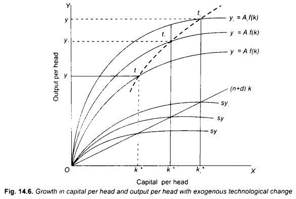
In general, if technological improvement ∆A/A per year is taken to be equal to g per cent per year, then production function shifts upward at g per cent per year as shown in Fig. 14.6 where to begin with production function curve in period t₀ is y₀ = A₀ f (k) corresponding to which saving curve is sy₀. With this, in steady-state equilibrium, capital per head is equal to k*₀ and output (income) per head is y₀. With g per cent rate of technological progress in period t_1, production function shifts to y₁=A₁ f(k) and correspondingly saving curve shifts upward to sy₁.

As a result, in period t₁, new steady state equilibrium capital per head rises to k*₁ and per capita output to y₁. With a further g per cent rate of technological progress in period t₂, production function curve shifts to a higher level, y₂ = A₂f (k) and associated saving curve shifts to sy₂. As a result, capital per head rises to k*₂ and per capita output to y₂ in period t₂. We thus see that progress in technology over time causes growth of per capita output (income). With this, aggregate output will also increase over time as a result of technological progress.

The neoclassical growth theory has been successfully used to explain increase in per capita output and standard of living in the long term as a result, technological progress and capital accumulation.