Solow’s Analysis of Growth | Economic Growth

The below mentioned article provides notes on Solow’s Analysis of Growth.

The Solow model shows how nations grow through the interplay of saving, population growth and technological progress.

Solow has proved conclusively that :

(1) capital formation,

(2) growth of the labour force and

(3) technological progress conjointly affect the level of an economy’s output and its rate of growth of per capita income over time. The primary importance has been assigned to the accumulation of capital.

Variables:

The Solow model focuses on four variables: aggregate output (Y), capital stock (K), labour force (L), and ‘knowledge’ or ‘effectiveness of labour’ (E).

Assumptions:

The focus of the Solow model is on the properties of the production function and the evolution of three factors of production (capital, labour and knowledge) over time.

The model is based on five assumptions:

1. The economy is closed and there is no government sector. So, in equilibrium, saving will equal investment; that is:

S = I

2. Secondly saving, S, are assumed to be proportional to income such that:

S = sY

where s is both the average propensity to save and the marginal propensity to save. It is assumed that 0 < s < 1.

3. The change in the capital stock (K) is equal to gross investment 1 less depreciation δK. Therefore the change of the capital stock over time is equal to investment less depreciation which is

K = I – δK

4. The labour force, L is assumed to grow at a constant exogenous rate of n, that is:

5. The fifth and final assumption is concerned with production technology. Suppose the aggregate production function is written as Y = F (K, L). The Solow model assumes a constant returns-to-scale production function. This means that multiplying both the inputs by say, λ, will give rise to an increase in output by λ, i.e., λY = F(λK, λL).

Capital Accumulation:

Solow’s analysis shows how growth in the capital stock as also in the labour force, and advances in technology — interacts in an economy and how these three factors affect a nation’s total output of goods and services.

The Supply of and Demand for Goods:

The supply of and demand for goods play an important — perhaps the central — role in the Solow model of growth. The reason is that from the supply of and demand for goods we can determine how much output is produced at any given time, as also the pattern of allocation of this output among various (alternative) uses.

Step 1: The Supply of Goods and the CRS Production Function:

The aggregate production function of the Solow model states that output (supply of goods) depends on the capital stock (K) and the labour force (L):

Y = F(K, L) … (7)

The production function is assumed to be homogeneous of degree one, i.e., it exhibits CRS, i.e.,

XY = F(λK, λL) …(7a)

for any positive number λ. Thus if we multiply both K and L by λ., Y also gets multiplied by λ,.

The assumption of CRS simplifies the analysis considerably. It enables us to analyse all quantities in the economy with reference to the size of labour force. If, for instance, we set λ = 1/L, the aggregate production (7a) becomes

Thus output per head — is a function of the amount of capital per head. Since the number ‘1’ is constant, we ignore it. The assumption of CRS brings into focus a very important point: The size of the economy, measured by the size of the labour force, does not affect the relationship between output per worker and per capita availability of capital.

Since the size of the economy does not affect the relationship between output per worker (Y/L) and the amount of capital per worker (K/L), we can express the production function as

y = f (k)… (9)

where y = Y/L, k = K/L and f(k) = F(k, 1). So the production function is expressed in per worker terms. Fig. 4.2 graphically represents the production function. Its slope is MPK = Δy / f (k + 1) – f (k).

The marginal product of capital (MPK) shows how much extra output is produced by using one extra unit of capital, the usage of labour remaining the same. The curvature indicates diminishing MPKAs more and more capital is used, lesser and lesser addition is made to the total product of the economy.

The production function indicates how the amount of output per worker y = f (k) is determined by the amount of capital per worker.

Step 2: The Demand for Goods and the Consumption Function:

The demand for goods consists of consumption and investment:

y = c + i … (10)

where y = output per worker, c = C/L consumption per worker and i = 1/L investment per worker.

This equation is the per-worker version of the national income identity for a two-sector closed economy without government.

The consumption function is of the following simple form:

c = (1 – s)y …(11)

where 5 is the propensity to save and 1- s is the propensity to consume (0 < s < 1). Although different public policies can influence the saving rate (s), Solow takes this as given.

If we substitute (1- s)y for c in equation (10) we get:

y = (1 – s) y + i or, i = sy … (12)

This means that investment is equal to saving (which is the product of the saving rate s and income per worker y). Thus, in the Solow model, the rate of saving (s) is also the production of output devoted to investment.

Growth in the Capital Stock and the Steady State:

The main determinant of the economy’s output, per period, is its capital stock. Economic growth occurs when capital stock increases over time. The size of the capital stock is determined by two opposite forces: investment and depreciation. While investment (expenditure on new plant and equipment) increases the stock of capital, depreciation (the wear and tear of old capital) reduces it.

By substituting the production function for y in equation (12), we get:

i = sf(k) … (13)

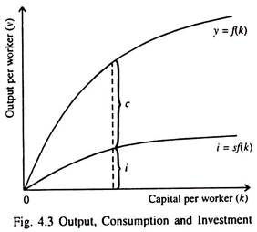
Equation (13) expresses investment per worker as a function of the capital stock per worker. This equation relates the existing stock of capital (k) to the accumulation of new capital (i). Fig. 4.3 shows the same relationship diagrammatically.

It shows two things at the same time: (i) how, for any given value of k, the amount of output is determined by the production function J(k), and (ii) how the allocation of that output between consumption and investment is determined by the rate of saving (s).

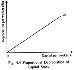
Solow assumes that a certain proportion (δ) of the existing stock of capital wears out every year and has to be replaced. Here δ is the annual rate of depreciation (or capital consumption). The amount of capital which depreciates each year is δ k. Fig. 4.4 shows the proportional relation between δ and k.

Thus we have:

Δk = i – δk = sf(k) – δk = sy – δk … (14)

i.e., the change in capital stock between one year and the next is the difference between investment and depreciation. From equation (14) we get Ak = sf(k) – 5k, since i = sf(k).

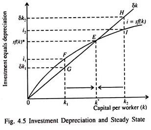
Fig. 4.5 slows the rate of investment and the corresponding depreciation rate for different levels of the capital stock (k). The larger the volume of capital, the greater the amount of output and invest­ment. At the same time the higher the capital stock the larger the amount of depreciation.

Fig. 4.5 shows that there is only one capital stock k* at which the amount of investment equals the amount of depre­ciation, so that there is no addition to the capital stock (i.e., Δk = 0, because i = sf(k) = δk at k*). This means that the capital stock (k) and output f(k) remain steady over time. Neither is growing nor falling. Therefore k* is called by Solow the steady-state level of capital.

Significance of the Steady State:

The steady state is significant for an important reason. Once the economy reaches the steady state it will stay there. This means that, regardless of the level of capital with which the economy begins, it ends up with the steady state level of capital. So the steady state represents, the long-run equilibrium of the economy. This point requires a little elucidation.

If the economy starts from a capital stock of k₁, which is less than k*, the capital stock will rise because the volume of investment exceeds the amount of depreciation. Over a number of years, the capital stock will continue to grow along with output f(k), and will, ultimately, reach the steady state level of capital per worker (k*).

The converse is also true. If the economy starts with more than the steady state level of capital, such as k₂, capital stock will continue to fall and will ultimately reach the steady- state level, at which investment equals depreciation. This will happen because capital stock is wearing out faster than it is being replaced, in which case the level of investment will fall short of the amount of depreciation. So in a steady state there is no pressure for the capital stock to either rise or fall.

Finding Out the Steady-State Capital Stock:

There are two ways of finding out the steady state capital stock. First, we can watch the progress of the economy for many years. The second method is theoretical.

We know that:

Δk = sf(k) – δk … (15)

This equation shows how k grows over a period of time. Since in the steady state the value of k is such that Δk = 0,

0 = sf(,k*) – δk*

or, equivalently, k*/f (k*) = s/δ…(16)

This equation enables us to calculate the steady-state level of capital per worker, k*.

Saving and Growth:

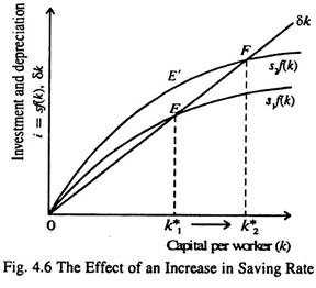
An increase in saving rate leads to an increase in the volume of investment and this, in its turn, leads to an increase in the growth rate. This point is illustrated in Fig. 4.6.

The economy starts with a steady state saving rate s₁ and capital stock k₁*. If now the saving rate increases from s₁ to s₂, the investment curve i = sf(k) shifts upward. At the original saving rate s₁, and the initial capital stock k₁*, the amount of investment is just sufficient to
offset the amount of depreciation.

As soon as the saving rate rises, investment auto­matically goes up. But, since both capital stock and depreciation remain unchanged in a steady state, equilibrium investment exceeds depreciation by EE’, As a result the capital stock continues to rise.

The process goes on until the economy reaches the new steady state, which has a larger volume of capital k*₂ and higher level of output compared to that in the old steady state. In short, an increase in the saving rate raises investment. This, in its turn, causes the capital stock to grow towards a new steady state, which is k*₂ and is greater than k* as shown in the above figure.

The Main Message of the Solow Model:

Thus in the Solow model the saving rate is the proximate determinant of the steady state capital stock. There is a positive correlation between s and f(k). If s is high k is also high and f(k) is correspondingly high. The converse is also true. This message has a very important implication from the policy point of view.

We know that government budget deficit and the corresponding public sector borrowing requirement (PSBR) can reduce national saving and crowd out (obstruct) private investment. In the context of the Solow model we can see the long-term consequences of a reduced saving rate, viz., a lower capital stock and a reduced level of GDP.

This is the main reason why many liberal economists — such as Milton Friedman and Edmund Phelps — are very much critical of persistent deficits in the government budget.

Relation between Saving and Economic Growth:

In the Solow model there is a direct relation between saving rate and growth rate. But the relation holds only in the short run. This means that an increase in the saving rate leads to faster economic growth only temporarily, i.e., until the economy reaches the new steady state. If the economy is able to maintain high saving rate, it also succeeds in maintaining a large capital stock and a higher level of output.

But it will not be able to maintain a high rate of growth for an indefinite period. One reason is diminishing marginal product of capital.

Theory and Practice:

A study of cross-section data shows that there is a strong association between investment rates and per capita output (income). High-investment nations grow much faster than their low-investment counterparts. But the correlation between the two variables is not perfect.

There must be other determinants of improved living standards such as investment in human capital (expenditure on education and training) and technological progress.