Cost Volume Profit Analysis: Definition, Example, CVP analysis, Assumptions, Break Even Analysis and Examples

C.V.P. analysis is a technique used to study the inter-relationship between costs, sales and net profit. It shows the net effect that fluctuation in cost, price and volume has on profits. The higher the volume of output, the lower will be the unit cost of production and vice-versa as the fixed overhead cost in total cost does not change with changes in the volume of output.

CVP analysis is thus the study of inter-relationship of cost behaviour, levels of activity and the resultant profit from each alternative combination.Each of these three variables involved in CVP analysis is influenced by a number of factors. The cost of a product is, for instance, influenced by factors such as cost of inputs, volume, size of plant, efficiency of production, product- mix, etc.

Contents

Introduction to Cost Volume Profit Analysis
Definition and Meaning of Cost Volume Profit Analysis
Objectives of Cost Volume Profit Analysis
Purposes of Cost Volume Profit Analysis
Assumptions of Cost Volume Profit Analysis
Applications of CVP Analysis in Various Situations
Uses of Cost Volume Profit Analysis
Measure for Volume of Activity in CVP Relationship
Presentation of CVP Analysis
Break Even Analysis, Break-Even Point and Break Even Chart
Profit/Volume Ratio
Margin of Safety
Angle of Incidence
Profit Graph
Limitations of CVP Analysis

What is Cost Volume Profit Analysis: Meaning, Definition, Examples, Profit Analysis, CVP Analysis, Objectives, Assumptions, Applications, Uses, Break Even Analysis, Margin of Safety and Examples

What is Cost Volume Profit Analysis – Introduction

ADVERTISEMENTS:

The concept of C.V.P. is relevant to virtually all decision-making areas.The managers use this technique extensively to determine B.E.P., Margin of safety, Profits /Losses at various levels of output, etc. It is an important tool of short term planning and forecasting of business activities and is useful in taking short-run decisions and formulating business policies.

Basic questions of interest to management decision making areas, e.g., what should be the volume for a desired profit, what changes in selling price affect profit position, what should be the optimum product-mix of the company, how variation of cost affects profit, etc., are answered by this analysis. C.V.P. analysis can be made with the help of equations, graphs, charts, etc.

Profit depends on many factors of which the selling price of the product sold, its cost of production and the volume of sales effected are most significant. Again, selling price depends to some extent on costs if a certain profit is to be earned, and volume of sales depends on volume of manufacture, which again is related to costs.

Cost depends on various factors, e.g., –

ADVERTISEMENTS:

(i) product-mix,

(ii) volume of manufacture,

(iii) internal efficiency or inefficiency in manufacture,

(iv) size of order,

ADVERTISEMENTS:

(v) variation of methods of production,

(vi) size of plant and

(vii) cost procedure followed (e.g., pricing of issues of materials, methods of recovery of overhead, method of wage payment, etc.).

Of all these, volume is the most significant factor. Volume often changes in business. When such changes occur due to outside factors management finds it difficult to control. C.V.P. analysis gives a complete picture of the profit structure which helps management to distinguish between the effect of sales, volume fluctuations and the results of price or cost variations on profit. It is an extension of marginal costing and uses the principles of marginal costing.

Cost Volume Profit Analysis – Definition and Meaning

The Official CIMA Terminology defines cost-volume-profit analysis as “the study of the effects on future profit of changes in fixed cost, variable cost, sales price, quantity and mix.” Accordingly, the objective of CVP analysis is to determine what will happen to financial results reflected in profit if a specified level of activity reflected in the volume fluctuates.

Similarly, the price of a product is influenced by such factors as market demand, competitive conditions, marketing policies, etc.The volume or the level of activity, in the short run, is dependent upon the existing production facility. Just as it takes time to expand output or the level of activity, it is equally so with regard to reduction in capacity.

Although it is true that none of the three variables can be singled out as the most important factor influencing the amount of profit, volume, is still the influencing factor. Short-run profitability will always be sensitive to sales volume.

CVP analysis is restricted to a period of one year or less. During this period, the output of a firm is limited to that available from the current operating capacity. Consequently, the analysis highlights the effects of changes in sales volume on the level of profits.

6 Main Objectives of Cost Volume Profit Analysis

(1) To forecast profit accurately, it is absolutely essential to determine the relationship between costs and profits on one hand and volume on the other. It aims at measuring variations in cost with volume.

ADVERTISEMENTS:

Profit planning considers the projected level of output, optimum product combination, estimated revenue, total cost of production and is thus based on C.P.V. analysis.

(2) C.V.P. analysis is used in setting up flexible budgets which show costs at various levels of activities.

(3) C.V.P. analysis helps management in the evaluation of performances for control purposes.

ADVERTISEMENTS:

(4) C.V.P. analysis may be helpful in formulating pricing policies by projecting the effect that various price structures have on costs and profits, especially when the demand for the product is elastic.

(5) C.V.P. analysis helps to ascertain the amount of overhead costs that could be charged to product costs at different levels of operation.

(6) It helps in making short-run tactical decisions, e.g., shift working, acceptance of special order, choice of sales-mix, etc.

Cost Volume Profit Analysis – Purposes

It analyses the relationship among cost, volume and profit and can be used for the following purposes:

ADVERTISEMENTS:

(i) To ascertain the amount of profit (or loss) at any level of activity.

(ii) To determine the selling price/sales volume which will give the desired amount of profit.

(iii) To ascertain the selling price/sales volume which will yield the desired return on capacity employed.

(iv) To determine costs and revenues at various levels of activity.

(v) To ascertain the effect of change (increase or decrease) in fixed costs, variable costs, selling price, production/sales volume on profit.

(vi) To suggest the change in sales mix for obtaining maximum profits.

ADVERTISEMENTS:

(vii) To compare profitability among products and firms.

Cost Volume Profit Analysis – 12 Important Assumptions

1. This analysis presumes that costs can be reliably divided into-fixed and variable category. This is very difficult in practice.

2. This analysis presumes an ability to predict cost at different activity volumes. In practice, a lot of experience may be required to reliably develop this ability.

3. A series of break-even charts may be necessary where alternative pricing policies are under consideration. Therefore, differential price policy makes break-even analysis a difficult exercise.

4. It assumes that variable cost fluctuates with volume proportionally, while in practical life the situation may be different.

5. This analysis presumes that efficiency and productivity remain unchanged. In other words, this analysis presents a static picture- of a dynamic situation.

ADVERTISEMENTS:

6. The break-even analysis either covers a single product or presumes that product mix will not change. A change in mix may significantly change the results.

7. This analysis disregards that selling prices are not constant at all levels of sales. A high level of sales may only be obtained by offering substantial discounts, depending on the competition in the market.

8. This analysis presumes that volume is the only relevant factor affecting cost. In real life situations, other factors also affect cost and sales profoundly. Break-even analysis becomes oversimplified presentation of facts, when other factors are unjustifiably ignored.

Technological methods, efficiency and cost control continuously influence different variables and any analysis which completely disregards these over changing factors will be only of limited practical value.

9. This analysis presumes that fixed cost remains constant over a given volume range. It is true that fixed costs are fixed only in respect of a given capacity, but each fixed cost has its own capacity. This factor is completely disregarded in the break-even-analysis. While factory rent may not increase, supervision may increase with each additional shift.

10. This analysis presumes that influence of managerial policies, technological methods and efficiency of men, materials and machines will remain constant and cost control will be neither strengthened nor weakened.

ADVERTISEMENTS:

11. This analysis presumes that production and sales will be synchronised at all points of time or, in other words, changes in beginning and ending inventory levels will remain insignificant in amount.

12. The analysis also presumes that prices of input factors will remain constant.The application of cost-volume-profit relationship is restricted by the assumptions on which it is based. Therefore, cost- volume-profit analysis cannot be used indiscriminately.

Practical Applications of CVP Analysis

CVP analysis is of immense utility to managerial personnel.

Besides being a tool of profit planning, the analysis has its practical application in the following situations:

(i) Forecasting and profit planning at different levels of activity;

(ii) Cost control through flexible budgeting;

ADVERTISEMENTS:

(iii) Managerial decision-making with regard to the volume of activity necessary for realising the profit target; estimated profit or loss at different levels of activity within the plant capacity; and the level of activity necessary for avoiding loss;

(iv) Guide to fixation of selling price; and

(v) Impact of cost on profit.

Cost Volume Profit Analysis – Top 6 Uses

1. This relationship enables management to predict profit over a wide range of volume. This knowledge is very useful in preparing flexible budget.

2. In a lean business season, company has to determine the price of the products very carefully. It becomes necessary sometimes to bring down the price to boost the sale of a product. For all decisions like this, management must determine, by cost-volume-profit analysis, what impact this reduction in price is going to have on profit position of a company.

3. Analysis of cost-volume-profit relationship helps in decision-making. There are situations when management has to decide whether it should add to its capacity or not. With the knowledge of cost-volume-profit analysis, a manager can easily take decision showing, in its report how utilization of available capacity will lead to increase in profit.

4. Analysis of cost-volume-profit relationships helps in evaluating profit performance.

5. Cost-Volume-Profit analysis helps in profit planning. Under profit planning, company first declares the profit that it wants to make during the ensuing year. Thereafter, sales level necessary to yield that profit is attempted.

Cost-volume-profit analysis helps in profit planning in the following ways:

(i) It helps in estimating income at a particular sales level.

(ii) It helps to determine change in profit due to change in sales volume.

(iii) It helps to execute the idea of profit planning. In other words, we arrive at the sales level to be attempted for a desired profit by the knowledge of relationship existing between cost, volume and profit.

(iv) It helps to find out the sales required to meet proposed expenditure.

6. The knowledge of cost-volume-profit relationship can be of substantial help in pricing. The studies based on cost-volume-profit relationship make it possible to visualise the probable results of proposed or expected changes on cost, volume or price. Companies are often tempted to reduce prices on existing products in an effort to increase volume.

This is done to spread fixed costs over a larger volume of production.For taking any decision for reduction of prices the management should know the relationship between decrease in price and increase in volume. Any price decision has to take into account short-run and long-run considerations, i.e., possibility of spoiling the market and the probable action of competitors.

Measure for Volume of Activity in CVP Relationship

In C.V.P. relationship study one must define volume or activity accurately.

Volume is generally expressed as:

(i) Direct labour or Machine hours;

(ii) Value or units of sales;

(iii) Sales capacity as a percentage of maximum sales;

(iv) Production capacity as a percentage of maximum production;

(v) Cost or units of production;

(vi) Direct wages.

The selection of appropriate volume index becomes difficult, especially when the problem is to select an overall index to relate all items of cost in a department or cost centre.

While selecting a measure for volume, the following points should be considered:

i. The selected base should be understood easily.

ii. When production can be expressed in units like tonnes, litres, kilograms, numbers, etc., such common physical unit may be chosen as the volume base or index.

iii. The index selected should be susceptible to sufficient control and it should not fluctuate frequently. Hence, standard labour hours will be a better base than actual labour hours.

iv. The index chosen should not be affected by factors other than volume.

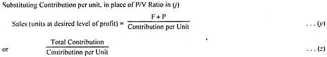
Presentation of CVP Analysis – Formula, Contribution and Equation

Cost-volume-profit relationship may be presented either mathematically or graphically. The mathematical method yields the required information more quickly than the graphical method. Besides, it is a flexible method also. While presenting the CVP relationship mathematically, it is necessary to make the assumption that selling price and variable cost remain constant per unit of output.

CVP analysis is an extension of marginal costing. In the context of marginal costing, it has been pointed out that sales revenue minus variable cost of sales gives us contribution to be applied for the recovery of fixed cost. Profit will then be the excess of contribution over fixed cost. This can be put in the form of a mathematical formula, known as the ‘Marginal Cost Equation’.

This formula is:

Sales – Variable cost = Contribution = Fixed cost + Profit

OR, Net profit = (Units sold x Price per unit) – (Units sold x Variable cost per unit) + Total fixed cost

OR, Sales – Variable cost – Fixed cost = Profit

OR, Sales = Variable cost + Fixed cost + Profit

OR, P = px-(a + bx)

Where P is the net profit, p is the selling price, x is the number of units sold, a is the total fixed cost, and b is the variable cost per unit.

Contribution:

Excess of sales revenue over variable cost is known as ‘contribution’. The Official CIMA Terminology defines this term as “Sales revenue less Variable cost of sales”. This may be expressed as total contribution, contribution per unit or as a percentage of sales. It is called ‘contribution’ as it initially contributes towards the recovery of fixed costs and thereafter, towards profit of the business.

This contribution is a ‘fund’ for both fixed expenses and profit.The contribution concept is based on the theory that profit and fixed expenses of a business constitute joint cost which cannot be equitably apportioned to different segments of the business. Hence, contribution serves as a measure of efficiency of operations of various segments of the business. Profit is the excess of contribution over fixed cost.

When put in the form of an equation:

Contribution = Fixed cost + Profit … (1)

OR, C = F + P

OR Sales (S) – Variable cost (V) = Contribution (C) … (2)

Putting (1) and (2) together, we get:

Sales – Variable cost = Fixed cost + Profit

OR, S-V = F + P

This is the fundamental marginal costing equation also known as the cost- volume-profit equation.

Break Even Analysis, Break-Even Point and Break-Even Chart

Break-even analysis is a widely used technique to study cost-volume-profit relationship. The narrower interpretation of the term break-even analysis refers to a system of determination of that level of activity where total cost equals total selling price.

The broader interpretation refers to that system of analysis which determines probable profit at any level of activity. It portrays the relationship between cost of production, volume of production and the sales value.It may be added here that CVP analysis is also popularly, although not very correctly, designated as “Break-even Analysis.”

The difference between the two terms is very narrow. CVP analysis includes the entire gamut of profit planning, while break-even analysis is one of the techniques used in this process. However, the technique of break-even analysis is so popular for studying CVP Analysis that the two terms are used interchangeably. For the purposes of this study, we have also not made any distinction between these two terms.

The cost of production, can be divided into fixed and variable costs, and at different levels of production, changes are bound to occur in such costs. The effect on profit on account of such variations is studied through break-even analysis.

Besides that in business, the selling prices of products are also changed from time to time. It is essential for business to know the impact of such changes on profits. Break-even analysis is a media to have an insight into these effects and thus helps in taking important managerial decisions.

Break-Even Point:

The point which breaks the total cost and the selling price evenly to show the level of output or sales at which there shall be neither profit nor loss, is regarded as break-even point. At this point, the revenue of the business exactly equals its cost. If production is enhanced beyond this level, profit shall accrue to the business, and if it is decreased from this level, loss shall be suffered by the business.

Break-even point is the point at which contribution is just sufficient to recover fixed costs; since whatever fixed costs are incurred in the business, these are absorbed by production till this point. Whatever production takes place beyond this level, it will yield additional contribution in the form of profit only. In other words, increase in contribution means increase in profit.

The break-even point can be expressed thus:

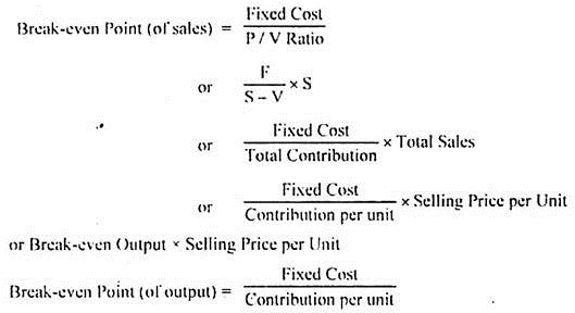
Fundamental Marginal Costing Equation and Equation to Derive Relevant Variables.

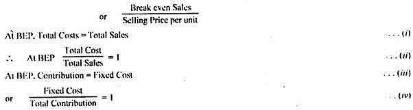
Fundamental Equation:

The fundamental marginal costing equation, out of which the different tools of marginal costing technique have been developed, is as under: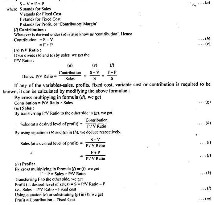

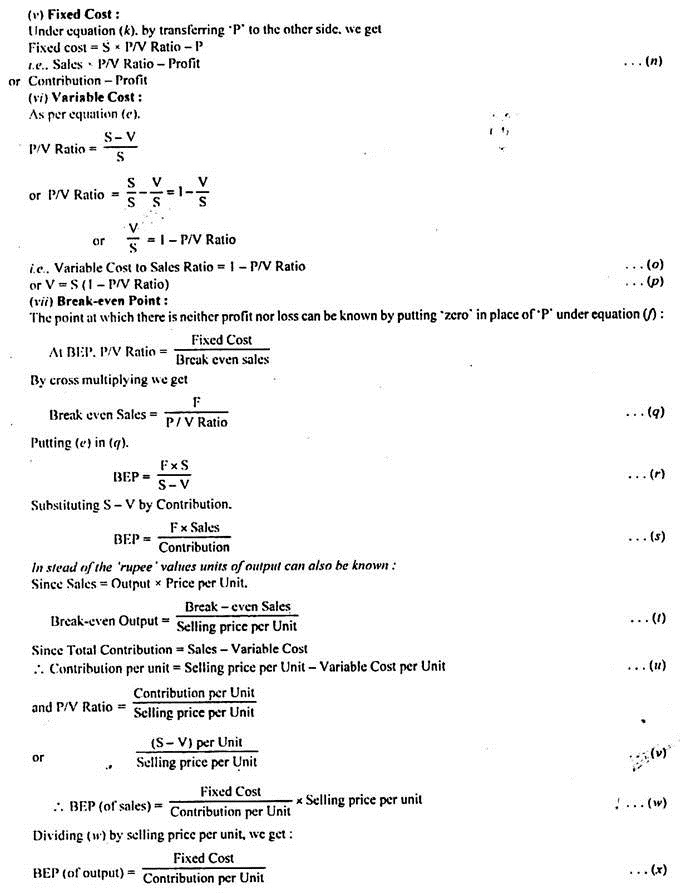
Observation:

The student needs to remember only the fundamental marginal costing equation. He need not cram all the equations. The desired equation can be derived by him, by self, simply be twisting the fundamental marginal costing equation.

However, the methodology, mainly mathematical, has to be understood by him, for purposes of application. There can be other derivations also from the above equations, to suit the particular requirements.

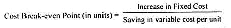
Cost Break-Even Point/Cost Indifference Point:

It refers to a situation where the costs under two alternatives is equal. It is also known as Cost Indifference Point. The point enables the firm to identify which alternative is better to operate at a given level of output or activity.

The cost break-even point can be computed as under:

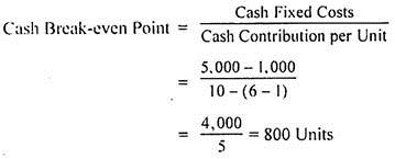
Cash Break-Even Point:

It is the level of output or sales where there will be “no cash profit and no cash loss” to the firm. In other words it is that activity level where the cash inflow will be just equal to cash required to meet immediate cash liabilities. For this purpose, the fixed costs are divided into two categories-

(i) Fixed Costs which do not require immediate cash outlay e.g., depreciation, deferred expenses, and

(ii) Fixed Costs which require immediate cash outlay, e.g., rent, salaries, etc.

The formula for its computation can be put as follows:

Cash Break-even Point (of Output) = Cash Fixed Costs/Cash Contribution per unit.

Example:

Selling Price per unit Rs. 10

Variable Cost per unit Rs. 6

Fixed Costs Rs. 5,000

Fixed costs include Rs. 2,000 as depreciation, 50% of which has been taken as variable cost and included in the variable cost per unit given above presuming an activity level of 1,000 units.

The Cash Break-even point can be calculated as follows:

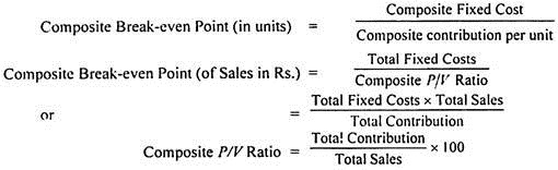
Composite Break-Even Point:

In case a concern is dealing in several products, a Composite Break-even Point can be computed according to the following formula:

Break-Even Chart:

The relationship between costs, profit and volume is best visualised by relating them on a chart called a break-even chart. It is also known as a profit-volume chart or graph. This term is rather more appropriate, since the term ‘Cost-volume-profit analysis’ is more suitable than the term ‘break-even analysis’.

The chart not only shows the point at which the costs and revenues would break-even, but also presents the costs, revenues and profits at various levels of output.The effect of changes in costs, selling price and volume of production can also be studied through this visual aid.

Accounting to the Chartered Institute of Management Accountants, London, the break-even chart is “a chart which shows profit and loss at various levels of activity, the level at which neither profit nor loss is shown, being termed the break-even point. This may also take the form of a chart on which is plotted the relationship either of total cost of sales lo sales or of fixed costs to contribution.”

Thus the break-even chart is a condensed pictorial representation of a master flexible budget, showing the normal profit for any given sales volume. It is a useful device for presenting a simplified picture of profit-volume relationships and to aid in demonstrating the effects of changes in various factors such as, volume, prices and costs. The chart impresses effectively and tells the entire story at a glance.

A break-even chart portrays:

1. Likely profits or losses a different levels of output;

2. The relationship between marginal costs and fixed costs;

3. The rate of growth of profit-earning for a convenient unit of output;

4. The break-even point;

5. The margin of safety;

6. The angle of incidence – The angle formed by the sales line and the total cost line at the break even point is known as “angle of incidence”. A high rate of profit is indicated by a large angle of incidence and vice versa.

7. The contribution and the P/V ratio (if desired).

Assumptions Underlying Break-Even Charts/Analysis:

While drawing break-even charts it is assumed that:

(i) Fixed costs remain constant at every level and do not increase or decrease with change in output.

(ii) Variable cost fluctuates directly with output. In other words they vary in the same proportion in which the volume of output or sales varies.

(iii) All costs are capable of being bifurcated into fixed and variable elements.

(iv) Selling price remains constant even with the volume of production or sales changes.

(v) Production and sales remain identical. Inventories do not change. They are kept either constant or at zero level.

(vi) There is only one product or a constant mix of product.

(vii) Costs are affected by volume only.

(viii) Periods are short enough that the time value of money is not important.

(ix) There will be no change in manufacturing methods and product specifications.

(x) Operating efficiency will not increase or decrease.

Advantages of Break-Even Charts/Analysis:

1. Provides detailed and clearly understandable information:

The chart visualises the information very clearly and a look at a glance shall give a vivid picture of whole affairs. The different elements of cost—direct materials, direct labour, overheads (factory, office and selling etc.)—can be presented through an analytical break-even chart. Further, the information presented is in a simple form and therefore is clearly understandable even to a layman.

2. Profitability of products and business can be known:

The profitability of different products can be known with the help of break-even charts, besides the level of no-profit-no-loss. The problem of managerial decision regarding temporary or permanent shutdown of business or continuation at a loss can be solved by break-even analysis.

3. Effect of changes of cost and sale prices can be demonstrated:

The effect of changes of fixed costs and variable costs at different levels of production on profits can be demonstrated by the graph legibly. Effect of changes in sales price also can be quickly grasped by the management by having a look at the break-even chart.

In other words, the relationship of cost, volume and profit at different levels of activity and varying selling prices is shown through the chart. Thus, it studies the requisites for survival of the company.

4. Cost control can be exercised:

The break-even chart shows the relative importance of the fixed cost in the total cost of a product; and if the fixed costs are high, they can be controlled by the management. Thus, it is a managerial tool for control and reduction of costs, elimination of wastage, and achieving better efficiency.

5. Economy and efficiency can be affected:

The capacity can be utilised to the fullest possible extent and economies of scales and capacity utilisation can be affected. Comparative plant efficiency can be studied on the break-even chart. The efficiency of output in plant is indicated by the angle of incidence formed at the intersection of the variable cost line and the sales line.

6. Forecasting and planning possible:

Break-even analysis is very helpful for forecasting, long- term planning, growth and stability.

Limitations of Break-Even Charts/Analysis:

1. Based on False Assumptions:

(a) Fixed costs do not always remain constant:

The assumptions underlying break-even charts do not normally hold good in every business concern. Fixed costs vary and do not remain constant at all levels of production. They have a tendency to rise to some extent after the production is increased beyond a certain level.

(b) Variable costs do not always vary proportionately:

The variable costs also do not always change in the same proportion as the volume of production or sales changes. Usually, the proportion increases if the law of diminishing returns is applicable in the business and it decreases if the law of increasing returns is applicable.

This presents difficulty in the drawing of the variable cost line (i.e., the total cost line) and the fixed cost line. The lines drawn are not straight and sometimes a curved line is obtained in respect of total costs.

(c) Sales revenue does not always change proportionately:

Besides the cost aspect, the sales revenue aspect is also not reliable regarding its non-variability at all levels of production. Selling prices are often lowered down with increased production in effort to boost up sales revenues. This gives a curved line in respect of sales revenue also in place of a straight line.

When both the total cost line and the sales line are not straight lines, the result produced, i.e., the break-even point may not show the correct level of output at which the total revenues can just recover the total costs and nothing more. It is also not correct to assume that with the maximum of output, the sales revenues will also be at the maximum level.

(d) Stock changes affect incomes:

The break-even chart depicts the volume of production of sales along the ‘X’ axis and thus ignores the effect of changes in stock volume. As a matter of fact, it is assumed that stock changes will not affect the income. But it is not true since the absorption of fixed costs depends on production and not on sales.

(e) Condition of growth not assumed:

Conditions of growth or expansion in an organisation are not assumed under break-even analysis. In the actual life of any business organisation, the operations undergo a continuous process of growth and expansion.

2. Limited Information:

Only a limited amount of information can be presented in a single break-even chart. If we have to study the changes of fixed costs, variable costs and selling prices, a number of charts will have to be drawn up.Similarly, when a number of products are manufactured, it would be a tedious job to present the information through a single break even chart.

However, the data can be shown by drawing several break-even charts; since through only one chart, the number of units sold cannot be measured along the ‘X’ axis. Besides that for complete analysis of a problem, the break-even chart has to be supplemented by various schedules and statistical material.

3. No Necessity:

There is no necessity of preparing break-even charts on account of the following reasons:

(a) Simple tabulation sufficient –

Even simple tabulation of the results of cost and sales can serve the purpose which is served by a break-even chart. Hence need of presentation through a chart and using the mathematical tool of break-even analysis does not at all arise.

(b) Conclusive guidance not provided –

No conclusive basis or guidance for action is provided to the management by the technique of break-even analysis.

(c) Difficult to understand –

The chart becomes very complicated and difficult to understand, particularly for a non-technical man, if the number of lines or curves depicted on the graph are large.

(d) No basis for comparative efficiency –

The chart does not provide any basis for comparative efficiency between different units or organisations.

Profit/Volume Ratio – Meaning, Equation and Limitations

The (profit/volume) ratio is better known as (contribution/sales) ratio.It is the contribution per rupee of sales. It can measure the rate of change of profit due to change in the volume of sales, as fixed cost remains the same in the short term period.

P/V ratio can be written as follows:

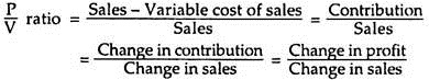
P/V ratio remains the same at different levels of activity. It is not affected by change in the fixed costs. A high P/V ratio indicates high profitability, whereas a low P/V ratio indicates low profitability. P/V ratio helps to compare the profitability of different sections of the business.

It helps to determine break-even point, profit at a given level of sales, sales volume needed to earn a given profit, profit for a given margin of safety, sales volume needed to maintain the present level of profit when selling price is reduced, profitability of products, processes or departments, etc.

From the above equation it is clear that P/V ratio can be improved if the numerator, i.e., contribution is increased. For increasing contribution either selling price is to be increased or variable cost is to be reduced.

Thus, improvement of y ratio can be done by any of the following ways:

(i) Increasing selling price;

(ii) Reducing variable costs by utilizing factors of production efficiently;

(iii) By changing the sales mix, i.e., selling more profitable products and, thereby, improving the overall P/V ratio.

Where profitability is high, increase of volume of sales is possible by spending more in advertisement and sales promotion.

Limitations of P/V Ratio:

The use of P/V ratio has the following limitations:

(i) P/V ratio leans heavily on excess of revenues over marginal costs.

(ii) P/V ratio does not consider the capital outlays needed by the additional productive capacity and the additional fixed costs, which are added.

(iii) It shows only the relative profitability of product lines which does not help to take a final decision.

(iv) The basic requirement for comparing profitability through P/V ratio is the proper separation of costs into fixed and variable components. Over-simplification may result in incorrect conclusion.

(v) Higher P/V ratio per unit of sales or per unit of production indicates the most profitable item only when other conditions remain unchanged.

Margin of Safety – Introduction, Formula and Examples

The difference between total sales and sales at break-even point represents the margin of safety. As the name indicates, it is the amount of sales above the break-even point. If there is fall in the sales to the extent of margin of safety, the firm will not be in the red. The higher the margin of safety, the better the situation. If a firm has a high margin of safety, it will continue earning profits even if there is a slight fall in the sales.

A high margin of safety provides strength and stability to the firm. A company should endeavour to keep its break-even point at the lowest level and, to maintain actual sales at the highest level. This is possible either by controlling fixed costs or by a dynamic sales policy or by reducing variable costs.Margin of safety can be expressed in absolute terms and also in terms of percentage.

In absolute terms, margin of safety is –

Actual sales – Sales at break-even point.

In terms of percentage, also called margin of safety ratio, it is commuted as under –

Example:

If actual sales of a firm are Rs. 60 lakhs and break-even sales amount to Rs. 45 lakhs, the margin of safety in absolute terms will be –

Actual sales – Sales at break-even point

Rs. 60 lakhs – Rs. 45 lakhs = Rs. 15 lakhs.

In terms of percentage, margin of safety ratio is –

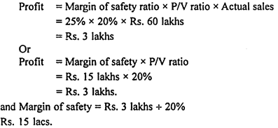
With the help of margin of safety ratio, profit can be determined as under –

Profit = Margin of safety ratio x P/V ratio x Actual sales

Conversely, Margin of safety = Profit ÷ P/V ratio

The above relationship indicates that once the break-even sales amount is achieved, contribution from all additional sales generates profits only.

Example:

Using the data and margin of safety in the above example and assuming P/V ratio to be 20% the profit figure can be ascertained as below –

Angle of Incidence – Meaning, Example and Graphs

Intersection of sales revenue line and total cost line creates an angle called Angle of Incidence. It is the indicator of the rate at which the company earns profit once it crosses the break-even point.

Though it is not possible to say, from the angle, the rate at which the company earns profit, it is possible to say whether it is at higher or lower rate depending upon the degree of the angle. Company with larger angle earns profit at a higher rate once it crosses the break-even point than the company with smaller angle of incidence.

This point becomes very obvious from the following example:

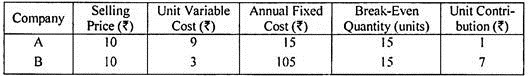
From the above figures, it is obvious that both the companies have to sell 15 units each to break-even. Once they reach the break-even point, Company A starts earning contribution (and therefore, profit) at the rate of Rs.1 on each unit sold over and above the break-even quantity. On the other hand, Company B starts earning contribution (and therefore, profit) at the rate of Rs.7 on each unit sold over and above the break-even quantity.

Hence, the difference in the size of angle of incidence is evident from the graphs presented below:

One noteworthy point is that company A is having a very small angle and company B, a very big angle.

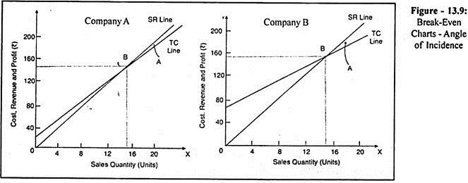
For the reasons cited above, companies work to achieve larger angle of incidence. Larger angle is an indication of higher P/v Ratio which in turn is an indication of lower Variable Cost Ratio. On the other hand, smaller angle indicates the lower P/v Ratio and therefore, higher Variable Cost Ratio. However, there is also another face to it.

This is relating to the angle left to the intersection point (i.e., break-even point). This indicates the rate at which the company’s profit declines if the demand falls below the break-even point. For instance, in the case of A company, if the demand falls below the break-even point even by one unit, the company incurs loss at the rate of Rs.1 a unit.

On the other hand, in the case of B Company, if the demand falls below the break-even quantity by one unit, it loses Rs.7 of contribution and therefore, the company has to incur loss at the rate of Rs.7 a unit. It is, therefore, obvious that the company with large angle of incidence earn more profit if they are operating above the break-even point and if they are expecting higher demand for products when compared to other companies with smaller angles of incidence.

On the other hand, in the case of the company operating below the break-even level and expecting a further fall in the demand, a small angled company earns more because it loses less.

Profit Graph – Steps, Multi-Product Profit Graph, Limitations and Uses

It shows the relationship between profit and volume of sales.

The steps for construction of profit graph are:

1. Select a scale for sales on horizontal axis. The sales line divides the graph into two parts.

2. Select a scale for fixed costs, profit or loss on the vertical axis. The fixed costs and loss are shown below the sales line on the left hand side vertical line and profit is shown above the sales line on the right hand side vertical line.

3. Plot the fixed costs and profits of corresponding sales and join them to get the profit line. The profit line is a diagonal line which cuts the sales line at break-even point.

Multi-Product Profit Graph:

When a company produces several products, management must know the y ratio of each product as well as for all products to maximise profit by selling products having higher ratios. A profit graph may also show the profitability of each product as well as the overall position of all the products taken together.

Limitations of Profit Graph:

1. Fixed costs are considered as constant irrespective of activity in the period which is not true.

2. A constant sales-mix is assumed where several products are sold.

3. Revenue and marginal costs are seldom linear over the full range of activity depicted; hence contribution line is not, in practice, a straight line.

4. It does not take capital employed into consideration.

5. It gives only a general static picture as it covers usually one year.

6. Changes in stocks do not affect the graph.

Uses of Profit Graph:

1. It helps to determine break-even point.

2. It helps to forecast costs and profits resulting from changes in sales volume.

3. It shows impact on profits of selling at different prices for a product.

4. It shows the deviations of actual profit from anticipated profit, relative profitability for high or low demand.

Limitations of CVP Analysis

CVP analysis is subject to the following limitations:

(a) All costs cannot be segregated into fixed and variable components;

(b) It is wrong to assume that volume is the only dominant factor influencing costs, while inflationary conditions and political factors also influence costs;

(d) The assumption of constant sales mix is also wrong since sales-mix changes with changes in demand;

(e) Where stocks are valued under absorption costing principles, profits vary with both production and sales. However, if they are valued under marginal costing principles, then profit will be the function of only sales; and

(f) The analysis assumes that costs and sales can be predicted with certainly. In point of fact, however, these are uncertain and hence, cannot be predicted with accuracy.