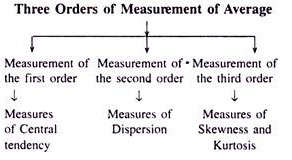
Meaning Central Tendency:
Many problems in economics and management involve frequency distributions. In frequency distributions, one encounters certain values that occur frequently while other values less frequently.
To be more specific, in many frequency distributions, the tabulated values show smaller frequencies at the beginning and at the end and larger or higher frequencies at the middle of the distribution.
This indicates that the typical values of the variable lie nearer the central part of the distribution and other values cluster or group around these central values. This behaviour of the data about the concentration of the values in the central part of the distribution is called central tendency (or location) of data.
A variable, as we know, possesses a number of observations which changes over time (called time series data) or space (called cross section data). If we examine the whole set of observations much carefully and quite intensively we find that these values have a general tendency to cluster around a central or a typical value existing almost in the central position. The particular value so identified is called the central value and the phenomenon is noted as the central tendency of the variable. Averages of several types computed are the usual measures of such tendency of a given variable.
ADVERTISEMENTS:
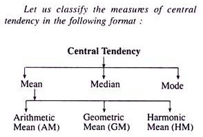
Usually, we are familiar with three following types of the central tendencies of a variable, namely—the mean, median and mode from the available values of the given variable. Again, means are of three categories—the Arithmetic Mean (AM) the Geometric Mean (GM) and the Harmonic Mean (HM).
We can represent them in the following way.
Classification of the Measures of Central Tendency of a Variable within a Particular Range of Variations:
We usually apply the following devises to quantify such tendency of a given variable appearing with a number of separate values:
Classification of Central Tendency:
(a) Mean:
(i) Arithmetic mean
(ii) Geometric mean
ADVERTISEMENTS:
(iii) Harmonic mean
(b) Median,
(c) Mode for grouped (having frequencies) and ungrouped (without having frequencies) data.
Summation Notation (∑):
The Symbol ∑ is the Greek capital letter sigma denoting sum. Let the symbol Xi (read x subscript i) denote any of the values X1 X2, X3… Xn, assumed by a variable x. The letter i stand for any of the number 1, 2…n is called a subscript.
Mean:
The mean or the arithmetic average of a set of values of a variable is the value obtained after dividing the sum of all the values of the given variable by their number.
The arithmetic mean is usually of two types:
(a) Simple arithmetic mean, and
(b) Weighted arithmetic mean.
ADVERTISEMENTS:
Simple AM:
The most commonly used measure of central tendency is the arithmetic mean. It is defined as being equal to the sum of numerical values of each and every observation divided by the total number of observations. In other words, it is calculated by adding together the values of the items in the set of observations and dividing the total by the number of items or observations.
The arithmetic mean is defined symbolically as:
ADVERTISEMENTS:
In equation (8.1), x (read x bar) is the mean or the arithmetic mean.
It is the representative value of all the observations given on a variable.
Example 1:
Find the average wage of the ten labourers working in a small industrial unit in a village:
ADVERTISEMENTS:
X: 88, 72, 33, 29, 70, 54, 86, 91, 57, 61
Solution:
The required sum of the wages of those ten labourers is:
It is clear from equation (8.1) or example 1 that if X1, x2 etc. occur with frequencies, say f1, f2 etc., then the AM becomes
ADVERTISEMENTS:
when N = ∑f is the total frequency or the total number of observations.
Example 2:
If the grades of 16 students in an examination were 55, 68, 36, 28 occur with frequencies 3, 2, 4, 6 and 1 respectively. Calculated AM.
Solution:
The Arithmetic Mean is Calculated on the basis of equation (8.2)
Example 3:
ADVERTISEMENTS:
The following marks are obtained by the Il-yr. students in a class-test out of 10. Score of one examinee was detected missing and included afterwards and the average calculated was 3. Determine the score of the last examinee.
1, 1, 0, 2, 0, 3, 0, 4, 8, 6, 5.
Solution:
Due to inclusion of one additional examinee in the process, the total number of examinees became 12 and hence their total marks should be 12 x 3 = 36.
Again, sum of the marks obtained by the previous 11 students was 30.
ADVERTISEMENTS:
Therefore, the score of the last one was
36 – 30 = 6.
Weighted AM:
The arithmetic mean attaches equal importance to all the items or observations. Truly speaking, all such observations may not attract same importance or weightage. Some observations may receive greater weightage compared to others. For example, greater weights are assigned to our daily needs (say, food) and lesser weights are given to luxury goods in our family budget.
Such importance attached to different items with figures (or numbers) according to their priorities is called weights. When the mean is expressed with respective weights one obtains weighted AM. This kind of mean is frequently used for studying various economic problems.
Note the similarity between the equations (8.2) and (8.3). Hence equation (8.2) can be considered as the weighted AM with weights f1, f2 …… fn.
ADVERTISEMENTS:
Example 4:
Find the weighted AM of the four given numbers 92, 125, 180 and 80 having their respective frequencies 12, 7, 6 and 9.
Solution:
The weighted AM of the four given numbers with their own frequencies can be expressed as:
Example 5:
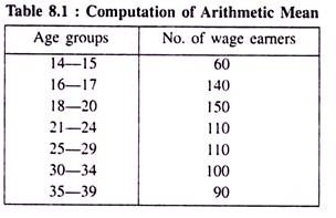
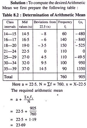
Compute the arithmetic mean of the following wage earning group of labourers.
Composite Mean from Two Separate Groups:
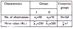
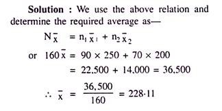
When two separate groups containing n1 and n2 observations with their respective arithmetic means x̅1 and x̅2 are given for a variable then the composite mean of those two groups together can be determined from the following relation:
x̅ here represent the composite or common mean for the two given groups together.
Example 6:
Calculate the composite mean of the salaries of the employees of two different departments of an organisation.
Table: 8.3: Calculate the Composite Mean
Important Properties of AM:
(a) Sum of a set of given observations is equal to the product of their number of observations and the AM.
Advantages and Disadvantages of AM:
According to the renowned statistician and author of this discipline G. U. Yule, arithmetic mean is a satisfactory average.
It has the following advantages:
(a) It is easily understandable.
(b) It is easily and exactly computable.
(c) It is suitable for algebraic treatment.
(d) It remains free from sampling fluctuations.
(e) Its calculation involves all the values of the given variable.
(f) It can rigidly be defined.
(g) It is safely usable and expressible in all situations.
However, arithmetic mean is not free from any disadvantages. Some of them are mentioned below:
(a) The arithmetic mean from a set of given observations is not identifiable only through observations.
(b) It is not correctly computable when a single observation is missing or rejected from the given data set.
(c) It can never be calculated correctly unless the entire observations on the given variable are supplied at a time.
(d) The arithmetic mean attaches greater importance to bigger items while smaller items receive lesser attention.
(e) It is to be kept in mind that it is not a locational average as such. It needs only mathematical calculations.
(f) Finally, the simple arithmetic mean suggests only a numerical figure and nothing else.
However, the arithmetic mean is a common type of primary statistical tool and widely used in various statistical analyses. Today, it is used as a very popular representation of central tendency of a variable and hence used frequently for several analytical purposes.
Meaning of GM:
The geometric mean like the AM is also a calculated average. However, it is another kind of statistical device to identify the central tendency of a variable having a finite number of observations. More precisely for a set of n-observations, it is determined as the n-th root of their product.
Symbolically, GM of the observations of a variable (x) having:
GM (for n-observations together of the variable x)of a set of n-positive numbers X1, X2….. Xn is the n-th root of the product of those numbers
It should be borne in mind that if the number of observations is more than 3, as demonstrated earlier, then computation becomes very difficult and tedious. In view of this kind of a problem, it is recommended to use logarithms. In other words, logarithms are used to simplify calculation when the number of observations is large enough. In order to calculate the GM we often use
If X1 X2 ….Xn occur with frequencies (or weights)f1, f2… fn respectively, the GM is then given by:
Advantages and Disadvantages of GM:
The geometric mean, like the arithmetic mean, has a number of advantages and disadvantages.
These are given in order below:
(a) It can be defined rigidly
(b) It is calculated on the basis of all the observations of a variable.
(c) It is much convenient to calculate required averages of ratios, rates, and percentages with the aid of GM.
(d) It is not affected by the exceptional and extremely large or small values of a variable.
(e) It gives the highest weight for the lowest observation and the lowest weight for the highest observation and thereby balances the entire procedure to get the best result.
(f) It is much suitable for using it in different mathematical treatments afterwards.
(g) It helps in the calculation for determining rates of exchange among the currencies of various countries.
Its disadvantages are noted below:
a. It is very difficult to calculate when the data is given in the fashion of a grouped frequency distribution having large frequencies in enough numbers.
b. The result becomes meaningless if any of the information is zero or negative.
c. The result finally obtained may not be equal to any of the observations given in the series.
d. It gives least importance to the marginal and extreme observations.
e. In some cases it cannot play the role as the true representative of an average.
f. It usually brings out the property of the ratio of changes and not the differences of change.
Computation of GM:
Example 1:
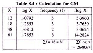
Find the GM of the observations 12, 18, 48 and 61 of a variable having their weights 5, 3, 2 and 8 respectively
Solution:
Let us prepare the data in the form of a table so as to calculate GM.
Example 2:
The GM of three numbers is 15 and the numbers are 5.25 and x, find the value of x-
Solution:
We know that for three numbers together-
Important Properties of the GM:
(a) When the observations on the given variable are equal in magnitude, the geometric mean will be equal to their common value.
Symbolically, we write:
XG = (C n)1/n = C
Here, the given variable x takes n-number of observations which individually are equal to C.
(b) The logarithm of the geometric mean of a set of values of a variable is the arithmetic mean of their logarithms.
(c) If y is a function of a variable x in the form y = ax, then the geometric mean of y is related to that of x in the similar form i.e yG= axG where yG and XG are the geometric means of y and X, respectively
(d) The geometric means of the ratio of two variables is the ratio of their geometric means:
(e) If there are two sets of values of a variable X consisting of n1and n2 observations and G, and G2 are their respective geometric means, then the geometric mean of the combined set is given by:
Meaning of Harmonic Mean:
The harmonic mean of a set of observations on a variable is defined as the reciprocal of the arithmetic average of the reciprocal of the given observations (any of the observations must not be zero).
If the variable noted is X which takes n- number of values as x1, x2, x3, … xn and their reciprocals are:
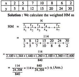
For the observations having their respective frequencies, the weighted HM can be computed as:
It is a special kind of average used in some selected situations.
Important Properties of the HM:
(a) If the given values of a variable are all equal (but ≠ 0) then their harmonic mean will be equal to their common value.
Here, n is the total number of observations of the variable and c is the common value.
(b) If a variable y is related to another variable X in the form y = ax, then the harmonic mean of y is related to that of x in the similar form:
(c) If n1 and n2 are two sets of values of a variable x and their respective harmonic means are H1 and H2, then the harmonic mean of the combined set (H) is given by:
Computation of the HM:
Example 1:
Calculate the simple harmonic mean of the numbers 3, 6, 24 and 48.
Solution:
Applying the principle of HM we get:
Example 2:
Determine the weighted HM for the observations of the variable X from the following:
Merits and Demerits of the HM:
Like all the devices of central tendency mentioned earlier, harmonic mean also has a number of merits and demerits.
These are:
Merits of the Harmonic Mean:
(a) It is defined much clearly and rigidly
(b) It is calculated on the basis of all the information available on the variable.
(c) It is very much suitable for using in various mathematical analyses.
(d) It remains more or less unaffected due to sampling fluctuations.
(e) It is easily computable and hence precise in nature.
(f) It always possesses a definite value.
(g) It considers smaller observation with larger importance and vice-versa.
(h) As it measures relative changes in the given observations of a variable, it becomes perfectly useful for finding out averages of certain ratios and rates.
Demerits of the Harmonic Mean:
(a) The result usually found has no existence in the given series of observations on the variable.
(b) It is not easily explainable, computable, and hence understandable.
(c) It is much restrictive in the sense that it cannot be calculated if any of the observations is zero.
(d) It has limited applications in practical situations.
Interrelationship among AM,GM and HM:
Let us consider the simplest example on a variable X having only two observations x1 and x2 (e.g., the two sides of a coin).
The same analysis can be extended for any number of observations on a variable and the same result can easily be established.
Other important relations are:
2. AM = GM = HM when all the observations on the variable are identical in magnitude.
AM > GM > HM for heterogeneous observations.
Symbolically, we generalise them as
AM > GM > HM
But, for any two different numbers the relation turns into:
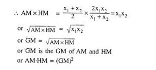
AM x HM = (GM)2
All the averages will become equal with each other when the variable assumes identical observations.
Median:
The median of a set of observations on a variable is identified as the middlemost value from those given set of observations. For a set of ungrouped data arranged either in ascending or descending order, the middlemost value or the median is calculated as the (N+1/2)-th-value for an odd number of observations. But, for an even number of observations, the median will be the mean of (N/2)-th and (N+1/2)–th value of those observations.
It is thus evident that the median divides the whole series into two equal parts. It is a positional average and is unaffected by the presence of an extremely large or small value. It can also be calculated from a grouped frequency distribution with open-end classes.
Example 1:
Find the median value of: Rs. 110, Rs. 90, Rs. 40, Rs. 50, Rs. 125, Rs. 65, and Rs. 100.
Solution:
Arranging the given values in ascending order, we obtain the sequence as Rs. 40, Rs. 50, Rs. 65, Rs. 90, Rs. 100, Rs. 110 and, Rs. 125. Thus, n = 7. Since 7 is an odd number. there is only one value at the middle which is the –th, i.e
the 4th value. Note that the 4-th valve = Rs. 90. Hence, by definition, the median value is Rs. 90.
Example 2:
Find the median of the values: 25, 24. 23, 32, 40, 27, 30, 25, 20, 10, 15, 45.
Solution:
Arranging the given values in the ascending order, we get the sequence as 10, 15, 20, 23, 24, 25, 25. 27, 30, 32. 40 and 45.
Thus, n=12, since the number 12 is even, it has two middle terms which are the 6-th and the 7-th terms, i.e. 25 and 25.
Hence, the Median by definition
This sort of calculation of the median value does not consider frequency distribution. Thus, the calculation for the median is nothing but simple for such a series.
Instead, we intend to calculate median for both ungrouped and grouped data. Let us consider the ungrouped data first. In this case, we first calculate cumulative frequencies corresponding to each value of the variable. Then the value of the variable corresponding to the (n+1/2) cumulative frequency is the median value where n = ∑f = total frequency.
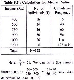
On the basis of example 3, we like to calculate cumulative frequency for ungrouped data (Table 8.5).
Example 3:
Find the median from the following data:
Solution:
How is cumulative frequency calculated has been shown in Table 8.5.
Example 4:
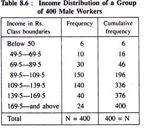
Consider the following income distribution of a group of 400 workers in a factory. Determine the median income.
Solution:
Note that the data are unequally spaced and open at both ends.
From the above table it is clear that the median must occur between Rs. 109.5 and Rs. 139.5 as N/2 = 200 occurs in between 196 and 336 as shown in the table. Hence median = Rs. 109.5 + a fraction of the class interval (109.5-139.5). This fraction may be found by simple interpolation.
We proceed as follows:
The difference in frequency from 196 to 336 corresponds to the difference in income from Rs. 109.5 to Rs. 139.5, i.e., corresponding to a difference of 140 in frequency there is a difference of Rs. 30 in income.
Therefore, corresponding to unit difference in frequency, there will be a difference of Rs.30/140 in income.
But, to find the median, we wish to proceed up to the cumulative frequency 200, i.e, to a difference of 200 – 196 = 4.
Thus, corresponding to a difference of 4 in frequency there will be a difference of Rs. 30/140 x 4 in income. Here Rs. 30/140x 4 = Rs. 0.85 is the fraction to be added. Hence, the median Rs. (109.5 + 0.85) = Rs. 110.35.
It is obvious from the above example that calculation of median from a frequency distribution with open ends does not produce any difficulty unless the median falls in an open x-class. We should also note that in finding out median for a grouped distribution, class boundaries, not class limits, should be used.
In interpolating the median value in the above example, we started from the top of the table, but we could have started from the bottom of the table as well and get the same result. Sometimes, it is stated that the median corresponds to the cumulative frequency equal to (n+1/2) where n is the total frequency.
This is true for raw ungrouped data with odd number of observations. But, for grouped frequency distributions this procedure should be avoided. Otherwise, the value obtained by interpolation starting from the top of the table will be different from the value obtained by starting from the bottom. This is not desirable because an average should uniquely be defined.
It should also be observed that whether we find mean or median from a frequency distribution, the values obtained will not be the same as those obtained from the raw data. This is natural because while making a frequency distribution our objective is to condense the data and the result of this condensation is the loss of some amount of information.
Example 5:
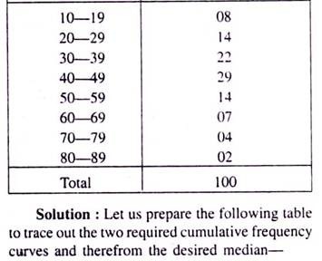
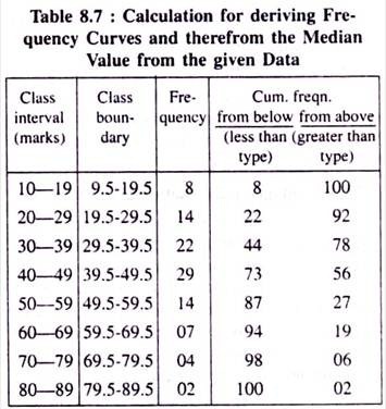
Represent the following data with the aid of cumulative frequency curves— (i) less than and (ii) greater than types and also determine the median value of the marks obtained by 100 students in Statistics:
Frequency distribution of marks obtained by 100 students in Statistics:
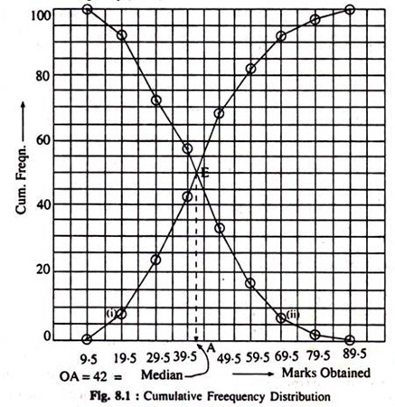
Now, we plot cumulative frequencies (of both the types) vertically and corresponding marks obtained horizontally on a two dimensional box diagram and easily trace out the two required cumulative frequency curves as shown below:
The two cumulative frequency curves (i and ii) are drawn from the given marks obtained by 100 students—(i) from below and (ii) from above.
We now find these two curves intersecting at point E and therefrom we get the median value for marks obtained by those 100 students as (39.5 + 02.5) = 42.0 (OA = 42)
Advantages and Disadvantages of Median:
In some cases the median has enough advantages over the arithmetic mean. If the set of observation contains a large value or a small value then the arithmetic mean may not give the correct measure. We know that the per capita income of an Indian is too low compared to the per capita income of an American. Same is true about the per capita incomes of rich people and the poor people of India also.
There exists a huge gap in income between the rich and the poor people. If incomes of the richer classes only go up largely without an increase in the incomes of the poor people, India’s per capita income will go up. But such higher per income cannot be called a true representative income. In such a situation, the median value of income will be a better representative of per capita income.
The median has the following merits and demerits:
Merits:
(a) It is simple to understand, explain, and easy to calculate.
(b) It is rigidly defined.
(c) It can be calculated for an open-end distribution.
(d) It is affected by the number of observations rather than the magnitudes of the observations.
(e) It remains unaffected from extreme values.
Demerits:
(a) It is not based on all the items of the series.
(b) It is not suitable for further algebraic treatment.
(c) It is not based on all the values as it is only a positional average.
(d) It is much affected from sampling fluctuations in comparison to the arithmetic mean.
Mode:
It is another effective statistical tool of measuring central tendency of a variable. For a set of observations on a discrete variable, a particular one which has the highest frequency is called its mode. The mode of a set of numbers is that value which occurs reputedly with the greatest frequency and in that sense, it is the most common value.
To make it simple, let us consider the following figures:
3, 5, 8, 5, 4, 6, 5, 9, 5
Here, the mode of these numbers is 5 because it has appeared the highest time (4 times) in the series of these numbers.
However, there may not be any mode for a series having no repetition of any particular number and for some other series two or more mode values can also exist, called bi-modal or tri-modal series. In most cases, we find a single mode in a series of numbers (or frequencies), we call it an unimodal frequency distribution.
Practically, it is easier to determine the mode value of a variable when it is discrete in nature compared to a continuous variable. For a continuous variable, its mode value is intimately related to the value at the peak point of its frequency curve. Hence, for such kind of a variable, the primary task is to derive the frequency curve from the given data and then identify its highest value corresponding to the peak point of the curve.
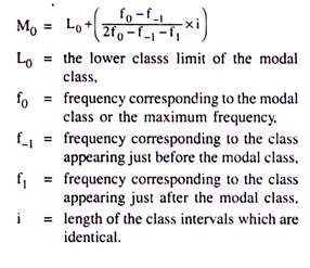
But, in a number of situations, we can determine the modal value of a variable without tracing out its frequency curve by using the following formula:
There exist two usual ways to calculate the mode value of a variable:
1. By drawing a frequency curve, and
2. By using the prescribed formula.
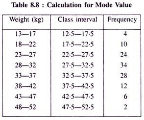
The method of calculation for the mode value from a grouped frequency distribution, as shown in table 8.9, may now be explained below:
Example:
Solution:
Observing the table closely. We find that the highest frequency is 34 and it is occurring within the class interval 28-32 where the class boundaries are 27.5-32.5.
We can now easily detect the following values as:
L0 = 27.5, f0 = 34, f-1 = 24, f1 = 28 and put them in the following formula:
Therefore, the required mode value is 30.62. In other cases, with unequal class intervals, the mode of the distribution can be determined through Karl-Pearson’s common relation established as Mean-Mode = 3 (Mean-Median), provided that the mean and the median are already determined.
Advantages and Disadvantages of Mode:
Mode is a useful measure of central tendency if the data provided are qualitative in nature. As mode is the value which has maximum concentration around, it has some distinct virtues.
Advantages:
(a) The concept of mode is easier to understand.
(b) It is not affected by the extreme values of the given variable.
(c) It is often determined by inspection only, at least from a simple frequency distribution. It is very often used in business.
(d) It is also calculable from a grouped frequency distribution with open-end classes.
Disadvantages:
However, the mode, as a measure of central tendency, is not free from any disadvantages.
These are:
(a) It is rather difficult to find out a well- defined mode in all cases.
(b) It is not based on all the values of the given variable.
(c) It is not suitable for further algebraic treatment quite readily and easily.
(d) It is significantly influenced by sampling fluctuations.
Essential Characteristics of a Good Statistical Average:
1. It should easily be understood and calculated. The AM is capable of easy calculation as compared to the GM or the HM. Further, the median as well as the mode have also simplicity in calculations.
2. A good average needs to be rigidly defined, i.e., the central value or the average value calculated should be unique in nature, otherwise the discretion in calculation of the average by the statisticians may creep in several errors afterwards.
3. It should be based on all the observations. For instance, only AM depends on all the observations. Median and mode do not have this attribute.
4. It should be capable of algebraic treatments in the sense that it should be capable of being used in further statistical computations.
5. It should not be influenced considerably by the fluctuations of sampling.
6. It should not be affected by the extreme values of the variable. Although median and mode are not affected by the extreme values, the AM is largely influenced by the extreme values—both large and small.
Thus, an ideal measure of average is very difficult to find out on several occasions.
Relation among Mean, Median and Mode:
The frequency distribution of a set of observations given on a variable are of two types—one is called the symmetrical or normal distribution where the mean, median and mode coincide with each other and the other is an asymmetrical one where of the mean, median and mode are different in magnitude, called skewed distribution.
In such skewed distributions, it is observed and established that they maintain a unique relation among them as:
Mean – Mode = 3 (Mean – Median),
called the Karl-Pearson’s relation.
Here, we can easily find out value of one when the other two values are already known. However, this relation can be safely applied only for unimodal and moderately skewed distributions.
Again, we find that both the mean and the median satisfy the conditions of right definition and stability but regarding their calculations numerically, the median is easier to calculate than the mean. On the contrary, the general fluctuations in sampling affect median to a larger extent than the mean, although certain exceptions are also there.
Regarding algebraic treatments of these devices for measuring central tendency of a variable, the mean is definitely the better one. In a situation where several series relating to one particular common aspect are combined together into one, we can find out the combined average from the separate averages of various series and their number of observations. But it can never be possible in the case of median.
For a set of given observations of a variable, the median, of course, has certain advantages over its mean. It is easily calculable and readily obtainable even without having the entire set of observations on the variable only when they are properly arranged.
Besides, in some special situations, mean cannot be calculated where the extreme class intervals are left unspecified (i.e., infinite) but the median can easily be obtained from them. In fact, in many cases, the median can appear as an ideal representative on the central tendency of the observations on a variable as it remains unaffected from its extreme items.
Further, it is agreed that the mean will surely be affected due to unavoidable sampling fluctuations but not the median and in that sense the median is recognised as a more natural average to represent the given observations on the variable than its mean.
From the above discussion, we can safely conclude that it will not be wise to select a particular one as the best from the available three measures of central tendency for the given observations on a variable in all situations. Actually speaking, depending on the nature and the quality of the data given and the objective of the study it is an important task for the user or the investigator and researcher to select the most suitable or the ideal one to meet his/her own purpose.
The mathematicians and the statisticians together, in this context, prescribe for ‘mean’ as the ideal one to accept in many cases than the other two. Specially, when the investigator is interested to conclude on a particular aspect provided with a given sample from its related population, the mean is undoubtedly the best one to select and use unhesitatingly.
