Law of Variable Proportions | Agricultural Economics

In this article we will discuss about:- 1. Introduction to the Law of Variable Proportions 2. Assumptions of the Law of Variable Proportions 3. Tabular Presentation 4. Three Stages.

Introduction to the Law of Variable Proportions:

Law of Variable Proportions examines the production function with one factor variable, keeping the other factors fixed. It refers to the input-output relation when the output is increased by changing the quantity of one input. When the quantity of one factor is varied, keeping the quantity of the other factors fixed the proportions between the variable factor and the fixed factor is changed.

Production in the short run is subject to the Law of Variable Proportions because some inputs are fixed in the short period and production can be changed only by changing the amount (proportion) of those inputs that are variable.

It states that as we go on increasing the amount of one factor, keeping amounts of the other factors of production constant, the return to the successive units of the variable factor are non-proportional: the return may rise at first, may be constant for a short while but must eventually diminishing. Therefore, this law is also identified as the law of returns as the Law Diminish Productivity, and as the Law of Non-proportional Returns.

As under this law we analyse the effects on output of variation in factor proportions, this is known as the law of variable proportions. The law of Variable Proportions is the new name for the “Law of Diminishing Returns”.

The law of variable proportions or diminishing returns has been stated by various economists in the following manner:

“As equal increments of one input are added, the inputs of other productive services being held constant, beyond a certain point the resulting increments of product will decrease, i.e., the marginal products will diminish.” (Stigler) “As the proportion of one factor in a combination of factors is increased, after a point, first the marginal and the average product of that factor will diminish.” (Benham)

“An increase in some inputs relative to other comparatively fixed inputs will cause output to increase; but after point the extra output resulting from the same additions of input will become less and less.” (Samuelson).

Marshall discussed the law of diminishing returns in relation to agriculture. He defines the law as follows:

“An increase in the capital and labour applied in the cultivation of land causes in general a less than proportionate increase in the amount of produce raised unless it happens to coincide with an improvement in the arts of agriculture.”

Prof Boulding is of the view that the expression “diminishing returns” is a loose one because it can be variously interpreted. He therefore avoids the use of the expression “diminishing returns” and names it ‘the Law of Eventually Diminishing Marginal Physical Productivity’ and defines it thus:

As we increase the quantity of any one input which is combined with a fixed quantity of the other inputs, the marginal physical productivity of the variable input must eventually decline.”

“If the input of one resource is increased by equal increments per unit of time while the inputs of other resources are held constant, total product output will increase, but beyond some point the resulting output increase will become smaller and smaller.” (Leftzvich)

“As more and more of some input, i, is employed, all other input quantities being held constant eventually at point will be reached where additional quantities of input, i, will yield diminishing marginal contributions to total product.” (Boumol)

“When total output or production of commodity is increased by adding units of a variable input while the quantities of other inputs are held constant, the increases in total production become, after some point smaller and smaller.” (Watson)

It is clear from the above definitions of the law of variable proportions (or the law of diminishing returns) that it refers to the behaviour of output as the quantity of one factor is increased, keeping he quantity of other factors fixed and further it states the marginal product and average product will eventually decline.

Assumptions of the Law of Variable Proportions:

The law of variable proportions or diminishing returns holds good under the following conditions:

(1) The State of Technology is given:

The state of technology is assumed to be given. If there is improvement in technology (inventions, streamlining of management) then MP and P may rise and the law may not work.

(2) There is only one Variable input:

One and only one resource is variable. It goes on increasing unit by unit.

(3) Other input must be Kept Constant:

There must be some inputs whose quantity is kept constant. It is only in this way that we can very the factor proportions and knows its effects on output. This law does not apply in case all factors are proportionately yarned. Beheaviour of output as a result of the variations in all inputs gives birth to “Returns to scale.”

(4) Variations in Proportions:

The law is based upon the possibility of varying the proportions in which the various factors can be combined. It does not apply to those cases where the factors must be used in fixed proportions. When the various factors are used in fixed proportions then the increase in one factor would not lead to any increase in output i.e., the MP will be zero.

(5) There is Short Period:

Short period has been assumed. In the long period all factors are variable and there are returns to scale and not the law of variable proportions.

Tabular Presentation of the Law of Variable Proportions:

The law of variable proportions can be easily grasped if we make use of a table. The following table gives hypothetical figures relating to the output of farm product. The inputs used is one unit of land and varying numbers of workers.

We are concerned with the different ratio of labour to land, not with the absolute quantities of labour and land. There may be any quantities of inputs. The proportion between the two must change. It is because of the change in ratio or proportion that the law is called the law of variable proportions. The product is in terms of quintals. We consider the product in physical terms and not in money terms.

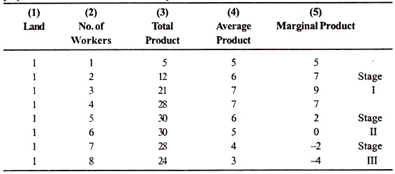
The product shown in the table is in respect of the workers employed on land. The farmer can vary the number of men to be employed on its cultivation. As he will change the number of men on the farm output will change.

The total product, average product, and the marginal product behave as shown in Table. At first as the number of men is increased from, 1 to 3, marginal as well as the average product increases. But as more men are employed the AP falls and the MP falls more speedily.

Fall of the average and the marginal product continues as more men are put on the farm. Hiring of the 6^th man forth if more men are added they will prove a nuisance to the already working men and will decrease production rather than increasing it; marginal product will become negative. The behaviour of the marginal product shows clearly three stages: first, it increases; second, it continues to fall; and third, it becomes negative.

The operation of the Law of variable proportion is diagrammatized in figure 6. As the quantity of the variable factor is increased relative to the fixed factors, total product increases. We can find out from this TP curve as to what is the position of the AP and the MP curves. AP of the variable factor with ON₁ unit employed is total product (KN₁) divided by the total units of the factor being used (ON₁).

Here the AP is the maximum and is equal to the MP. The increments to total product made by employment of additional units, of the variable factor continue to increase till the last unit on N₁ (Marginal product continues to increase).

After point K, total product increases all right but the rate of increase becomes less and less, that is the marginal product becomes less than the average product, and average product, after attaining a maximum at the point M, starts declining.

The marginal curve always falls faster than the average curve. Total product is the maximum (PN₂) when ON₂ units of the variable factor are employed. Henceforth if more units are employed total product declines or what is the same thing, marginal product becomes negative.

Bober says, “However, the most telling aspect of the law of returns lies in the eventually declining marginal product.” Thus it is the marginal product that is important when we have to take decisions about the employment of any input. When we talk of diminishing returns, we really mean diminishing marginal returns.

An examination of the table brings home to us the relationship between Average product and marginal product (average-marginal relations).

This relationship is reduced to three propositions given below:-

1. In the beginning marginal product increases, so does average product.

But marginal product (MP) is greater than average product (AP).

MP > AP

2. When average product is maximum and constant, marginal product is equal to it.

MP = AP

3. Eventually both the marginal product and average product fall; but marginal product is less than average product.

MP < AP

We can state the relationship in a slightly different language. When AP is increasing, MP is greater than AP. When AP is maximum and constant, MP is equal to AP. When AP is decreasing, MP is less than AP.

Three Stages of the Law:

The behaviour of these total, average and marginal products consequent on the increase in the variable factor is generally divided into 3 stages which are described below:

The three stages of the law of variable proportions are easily identified in the diagram. (Fig. 7)

Marginal product increases as we employ more units of the variable factor till ON₀ unit are employed. This is the first phase of the law popularly called the stage of increasing returns.

If we add more units, marginal product starts falling but average product rises so long as marginal product is above it. They are equal (SN₁) when ON₁th units are employed. Here the first Phase of the law of variable proportions, the stage of increasing returns, is over. Point N₁ corresponds to the maximum AP.

The second phase of this law starts with the employment of more units after ON₁ AP as also the MP starts falling. The ON₂ unit of the variable factor has an MP which is zero. The second stage of his law is what used to be called the Law of Diminishing Returns.

The third stage starts after the employment of ON₂ units. If more units are added, they have an MP less than zero. The additional units of the variable factor are not only redundant but harmful also, since they hinder rather than help production. In other terminology, point N₂ corresponds to the intensive margin beyond which production will not take place.

The Stage of Operation:

It is clear that a producer’s rational decisions can lie in stage II only. In stage I, the AP increases as more units of the variable factors are employed. The producer’s profit out of the employment of the factor continues to increase until the employment of ON₁ units.

There is incentive for the producer to expand production to employ the factor up to ON₁ amount. A rational producer will not produce such quantities of production as employ amount of the factor less than ON₁. As the second stage starts, MP starts falling. Falling MP is not any worry for the producer unless the MP becomes less than the MC of procuring the additional unit of the factor. The producer can decide the employment of the factor within stage II only.

We can rule out the equilibrium of the producer in stage I. Similarly employment of amounts of the factor as to reach stage III is out of the question. In this stage, the MP of the variable factor is negative while we can expect the cost variable factor to be always positive.

If the producer operates in this phase he adds to his costs while it lowers his production. No rational producer will do so. Therefore, a producer always decides the employment of a factor within the second stage. Exactly at what point he will stop further employment depends upon the price he has to pay for it.

Why Increasing Returns (Stage I)?

To begin with the quantity of the fixed factor is abundant relative to the quantity of the variable factor. When more and more units of the variable factor are added to the given fixed factor, the fixed factor is more intensively used. Thus as more units of the variable factor are put to work with an indivisible fixed factor, output increases rapidly due to fuller and more effective use of the latter.

Another reason why increasing returns appear at the initial stage is that as more units of the variable factor are employed the efficiency of the variable factor increases. This is because when there is a sufficient quantity of the variable factor, it is possible to introduce specialization which results in increased productivity.

Why Diminishing Returns (Stage 2)?

Why we get diminishing returns after a certain amount of the variable factor has been added to the fixed factor. Increasing returns appear in the first stage because of the more efficient use of the fixed factor as more units of the variable factor are employed to work with it.

Once the point is reached at which the amount of the variable factor is sufficient to ensure the efficient use of the fixed factor, then further increases in the variable factor will cause MP and AP to fall because the fixed factor then becomes inadequate relative to the amount of the variable factor.

We know that the production is the result of the co-operation of various factors assisting each other. In stage I, the fixed factor is abundant relative to the variable factor and former provides much assistance to the latter. In stage 2, on the other hand, the fixed factor becomes scarce in relation to the variable factor so that as the units of the variable factor are increased they receive less and less assistance from the fixed factor. As a result the MP and AP of the variable factor fall during the stage 2.

The law of diminishing returns, like that of increasing returns, stands upon the indivisibility of the fixed factor. There will be a level of employment of the variable factor at which indivisible fixed factor is being fully used and therefore the AP is maximum. It will happen where the variable factor has increased to such an extent that the fixed indivisible factor is being used in the optimum proportion with the variable factor.

Once the optimum proportion is disturbed by further increases in the variable factor, returns per unit of the variable factor will diminish because the indivisible factor is being used too fully. If the factors were perfectly divisible then there would not have been the necessity of taking a large amount of the fixed factor in the beginning to combine with the varying amount of the other factor.

In the presence of perfect divisibility, the optimum proportion between the factors could have got in very case. Prof. M.M. Bober rightly remarks, “Let divisibility enter through the door, law of variable proportions rushes out through the window.”

Mrs. Joan Robinson holds that the diminishing returns occur, because the factors of production are imperfect substitutes for one another. Thus Mrs. Joan Robinson remarks, “What the Law of Diminishing Returns really states is that there is a limit to the extent to which one factor of production can be substituted for another, or, in other words, that the elasticity of substitution between factors is not infinite.

If this were not true, it would be possible, when one factor of production is fixed in amount and the rest are in perfectly elastic supply, to produce part of the output with the aid of the fixed factor and then when the optimum proportion between this and other factors was attained to substitute some other factor for it and to increase output at constant.” We find therefore that law of diminishing returns operate because the elasticity of substitution between factors is not infinite.

Why Negative Returns (Stage 3)?

The phenomenon of negative returns in stage 3 is due to the fact that the number of the factor becomes too excessive relative to the fixed factor so that they get in each other’s way with the result that the total output falls.

Besides, too a large number of the variable factors also reduce the efficiency of the fixed factor. In the first stage, MP of the fixed factor was negative due to its abundance; in the third stage the MP of the variable factor is negative due to its excessiveness.

Section B: Factor-Product Relationship (How Much To Produce)

We have so far explained the main features of an increasing decreasing production function, the relationship between the total product, the marginal product and the average product in case of such a production function and the three stages of production as they appear in such a production function.

We shall now make use of this production and its three stages of production to decide how much a farmer should produce if he is to maximize his profits. In other words, we shall try to determine the conditions which govern factor- product relationship especially with reference to a situation of perfect competition-the market structure relevant for agriculture.

We may have a look at the following diagram.

The diagram shows the increasing decreasing production function (showing the movement of the total product and the three stages of production). However, in the present diagram, the total product has been expressed in value terms (TVPx) i.e. TPPx multiplied by the price of the product price which is constant under conditions of perfect competition.

As every point showing total physical production in the increasing decreasing production function has been multiplied by the same price, the shape of the total value product curve will exactly be a replica of the increasing decreasing function expressed in physical terms. All other relations i.e., those between total product, marginal product and average product will also remain unchanged. The division of the production function into three stages will also be at the same level input use.

We had to express the physical output as indicated by the increasing decreasing function in money terms because it is necessary that for determining profits and their maximum level, both the output as well as the cost should be in money terms.

There is another line OC in the diagram, starting from the origin. This line shows the total cost of the different amounts of input used (as shown on X-axis). At any point on this line, its slope is equal to the price of one unit of input.

The total cost function has been represented by an upward sloping line OC simply because the price of the input remains unchanged due to the assumption of perfect competition and each point on it is represented by the value obtained by multiplying the units of input used, with the constant price of the input.

Now, we are in a position to determine the point showing the maximum profit. We know that the profit is maximum where the gap between the total revenue and the total cost is the maximum or where the tangent to the total revenue curve is parallel to the tangent to the total cost curve.

If the present contest, we can treat the TVPx curve as representing the total revenue curve (the only difference in this case, from the total revenue curve used in common marginal analysis is that on X-axis, we have shown the amount of input used, rather than the output produced through it). The gap between the two is maximum at point F on the TVPx curve (i.e., at L on X-axis.) So, our conclusion will be that OL units of input (falling in the second stage of production) should be used if profit has to be maximised.

Section C: Factor Relationship (How to Produce)

We have already explained that a farmer who produces more than one crop on the one hand and uses, on the other, more than one variable input to produce a given crop has to satisfy conditions regarding three relationships.

We have so far discussed the conditions regarding factor-product relationship. In this section, we shall be considering those conditions which guide a farmer in deciding about the combination of various inputs necessary for producing a particular amount of a crop which, given the prices of various inputs, cost him the least. In other words, we shall be discussing the conditions governing factor-factor relationship.

In this analysis, for the sake of simplicity, we assume that only two variable inputs are required to produce a given crop. We also assume that perfect competition prevails and therefore, both the prices of inputs as well as of the output are constant, irrespective of the amount of inputs used or of the amount of output produced.

The Production function:

We must remember that whether it is the factor- product relationship or the factor-factor relationship or even the product- product relationship, the production function for the relevant crop will continue to be the starting point for our analysis.

The difference will lie only in whether it is a single input production function or a multi-input production function which is to be taken into consideration (we are considering one input or two input production functions for simplifying the analysis. In actual practice, however, single or even two input production functions are rather uncommon).

Whereas the indifference curves relate to consumption (utility), the isoquants relate to production. As such, the isoquants have all the properties which the indifference curves have viz., a higher isoquant represents a higher amount of production, two isoquants never cut or touch each other, the isoquants are normally convex to the origin and these slope downwards to the right etc. (It may be noted that isoquants for certain production function may be circular in shape. However, even in those cases, as we shall see later, in the region of rational production, the isoquants slope downwards to the right and are convex to the origin.)

Two of the above mentioned properties of isoquants need further explanation. Such an explanation is necessary for deriving the conditions necessary for minimization of the cost of production of a given output.

These properties of the isoquant are:

An isoquant slopes downwards to the right and is convex to origin.

The first part of this statement is quite obvious. It is assumed that both the inputs taken individually make a positive contribution to output. That is to say that an increase in any input will increase the total output. Under such conditions, if we increase one of the two inputs in a combination being used to produce a given output, we must reduce the amount of the other input if we want that the total output should remain unchanged.

If all the combinations required to produce a given output are obtained in this manner i.e., by increasing one input and by decreasing the other, the diagrammatic representation of these combinations will give a curve (an isoquant) sloping downwards to the right.

Reason for Convexity of the isoquant (to the origin):

In general, an isoquant is convex to the origin. The reason for this lies in the fact that the marginal productivity of each input taken in isolation decreases as its amount is increased. Suppose, with this assumption, we increase the amount of input x₂ in the combination used to produce a given amount of a commodity.

We must decrease the amount of the other input i.e., x₁ to such an extent that addition in output brought about by the increase in x₂ is exactly neutralized by the reduction of input x₁ Suppose this process is continued for finding out other combinations of x₁ & x₂ which produce the given amount of output. As x₂ is successively increased, less and less amount will be added to the total output by its increase.

As such, less and less of x₁ input will be given up for neutralizing the addition in output caused by the increase in x₂ In fact, the amount of x₁ to be given up will be still less because with each successive reduction in its amount, its marginal productivity will be raising. In other words for every successive increase in x₂ the amount of the other input i.e., x₁to be given up for keeping the total output at the same level, will successively decline.

In economic terminology, we say that the marginal rate of technical substitution goes on declining. And if the various combinations of two inputs resulting in the production of the same output reveal a declining rate of technical substitution, these combinations when plotted will always give a curve (isoquant) which is convex to the origin. The following schedule gives a tabular explanation of what we have pointed out just now.

The above table shows the declining marginal rate of technical substitution. We have already explained the reason for the declining marginal rate of substitution.

Diagrammatically, an isoquant with a declining marginal rate of technical substitution, will appear like a curve convex to the origin as shown below.

It is clear from diagram 9 that the marginal rate of technical substitution i.e.,declines as x₂ successively increases. And this accounts for the convexity of the isoquant. It is also clear from the above analysis that for any isoquant, the marginal rate of technical substitution at any point is equal to the value of its slope i.e., (or )at the point.