Game Theory II: A Close View

The below mentioned article provides a close view on the game theory II.

Two Person Zero Sum Games:

Having seen the basic tools of Game Theory, we can now look at some more specific examples.

The first case that we will look at is that of two person zero sum games. As the name suggests, the game involves two players. The zero sum is, because, in these games, the sum of the payoffs of the 2 players is zero. This means that, whatever one player gets, the other player gets the reverse.

For example, the game of matching pennies is a two player zero sum game. In this game, two pennies are flipped. If the two pennies are both heads or both tails, then player 1 wins the other player’s penny. If the two pennies land as opposites, then player 2 wins.

Thus, the payoff matrix for matching pennies is:

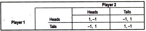
Often, two player zero sum games can be written as a simple matrix, since player 2’s payoffs are simply the negative of player l’s payoffs.

Thus, the above game could be written as:

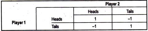
By looking for a Nash Equilibrium in the game of matching pennies (or any other non- constant¹, two player zero sum game) we will not find one in pure strategies. This is because whatever player 1 plays, player 2 loses. Thus, in all cases, either player 1 has the incentive to deviate to win more (or lose less), or player 2 has an incentive to deviate, to lose less (or win more).

‘By non-constant we mean that the payoff should not be the same for all outcomes. If the payoff for all outcomes is the same, then each outcome is a Nash Equilibrium,’ since neither player gains by deviating from a given strategy pair. We have seen that for zero sum games, there does not exist a Nash Equilibrium in pure strategies. However, the game may still have a ‘value’ or an equilibrium.

Sequential Games:

We begin by looking at zero sum sequential games. Consider the following game:

We analyse the above game using Zermelo’s algorithm (backward induction). This algorithm tells us that we should take a given sequential game and analyse it backwards. Therefore, we take each of the final decision nodes and choose the option that the player would choose at best for himself if he were to find himself at that node.

For example, at player 2’s final decision node, he can choose between a payoff of -4 or -6. He will choose -4 since this is best for him.

We show this decision by a darkened line. Once all the final nodes are analysed, we move back one stage and analyse these decision nodes. Here (at player 2’s only other decision node) he has the choice between -3 and -4. He will choose -3. Finally, we can see that player 1 will play such that he gets 3, since this is greater than 0.

Thus, by following their optimum strategies, the players will get 3 and -3, respectively. Thus, we call 3 the ‘value’ of the game, since this is its equilibrium outcome.

A Nash Equilibrium can also be calculated using Zermelo’s algorithm. In the above example, the Nash Equilibrium is the strategy that gives the payoff 3, but also includes the optimum choices at nodes that are not on the optimal path.

In other words, if all the choices at the nodes are left or right, the Nash Equilibrium is (left, left, right, right, left). This shows the optimal choice at each of the decision nodes, even if they are not reached by the optimal play of the game. Thus, backward induction can give us the Nash Equilibrium.

Constant Sum Games:

A constant sum game is one where the sum of the payoffs is the same for all strategy pairs:

The above game is one with a constant sum of 6. This is because the sum of the payoffs under each outcome is 6. Such a game can easily be converted to a zero sum game without changing the analysis of the game. The conversion can either be by removing 6 from player 1’s payoffs or by removing 6 from player 2’s payoffs.

Thus, the game becomes:

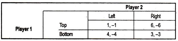
Thus the result for zero sum games hold true for constant sum games. However, we must remember to add 6 to player 2’s payoff when stating payoffs in our analysis.

Minimax and Maximin:

Since, simultaneous move zero sum and constant sum games do exist in real life, we need to develop some tools to give us an insight into what the outcome will be. For this reason, the minimax and maximin ideas have been developed.

Consider the following game:

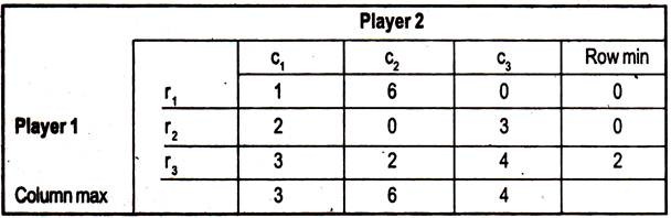
To work out the minimax value for player 1, we take the maximin values from the columns and we, then, select the minimin value from the column minima.

Minimax = min (column maxima) Similarly, to work out the maximin values we work out the row minima and we, then, take the maximin of these values.

Maximinm – max (row minima):

The minimax value will always be greater than or equal to the maximin value. If the minimax equals the maximin, the game is said to have a saddle point at this strategy pair.

Dominated Strategies:

Often in a game, a player has many strategies to choose from and this can be quite a complex task. However, we know from real life that when faced with certain situations, there are often some options which are definitely inferior to other options, regardless of what else happens.

For example, it is obviously bad to drive with your eyes closed, irrespective of what other drivers choose to do. For this reason, we will always choose to drive with our eyes open.

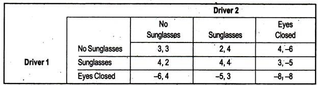
Looking at driver l’s options we can see that it is always better for him to drive with sunglasses rather than drive with his eyes closed, since the payoffs are higher, regardless of what driver 2 does. Thus, we can say, the strategy of driving while wearing sunglasses dominates the strategy of driving with your eyes closed. The same can be said for driver 2.

After eliminating the dominated strategies the game becomes:

The game can now be analysed to show that a Nash Equilibrium exists at the strategy pair (sunglasses, sunglasses).

N-Player Games:

Until now we have only analysed games in which there are two players. However, there are many instances when there are games with many players. For example, most races have more than two competitors, oligopolies with more than two firms, a league with many teams, etc.

To continue analysing these situations with the models we have seen so far would mean that we would need to work in 3-D, 4-D and N-D matrices. Since this is a very abstract and complex way of proceeding, we simplify our analysis by making a simple assumption.

We assume that all players in the game, except one, act as a single player would act. Thus, in an oligopoly situation, we take firm 1 to be player 1 and all the other firms in the industry to be player 2. Thus, we can analyse from firm 1’s point of view what its best course of action would be.

Example:

Consider an oligopolistic industry with five firms which produce text books, where price is the strategic variable and price decisions are taken simultaneously. If all the firms charge a low price, then each firm in the industry makes a profit of 2 lakhs. If all the firms charge a high price, then each firm makes a profit of 4 lakhs.

If one firm were to charge a low price while others charged a high price, they would make a profit of 5 lakhs, while everyone else made profits of 1 lakh. If one firm charged a high price while others charged a low price, the high price firm would make loss of 1 lakh, while everyone else made profits of 4 lakhs.

Write down the bi-matrix for this game, stating clearly who each player in the game represents. Find the Nash Equilibrium in the one shot game. Find the Nash Equilibrium in the infinitely repeated game, with no discounting.

Solution:

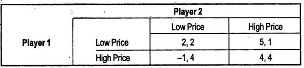
In this game, player 1 represents firm 1. Player 2 represents ms 2, 3, 4 and 5. The payoffs given are for firm 1 and for the other firms. For example the payoff-1, 4 means that firm 1 makes a loss of 1 lakh, while each of the other four firms makes a profit of 4 lakhs.

The Nash Equilibrium in the one shot game is Low Price, Low Price. The Nash Equilibrium in the infinitely repeated game could either be (Low Price Low Price) n-times or (High Price, High Price) n-times. This is because there is no incentive to deviate from either policy.

Game Theoretic Model of Entry Deterrence:

Firms in an oligopoly or a monopoly will try to maintain their market status by engaging in entry deterrence to avoid extra competition in their market. However, with many induce the profits to be made are very lucrative and new entrants would want to enter the market if possible. It is therefore, in a monopolist’s or oligopolies’ best interest to deter entry into the market.

Consider the following game:

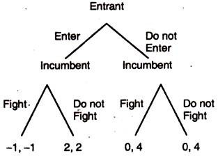
In the above game, the Nash Equilibrium can be shown to be Enter, Do not Fight, Do no Fight. However, this solution is not optima, for the incumbent firm as it would prefer a payoff d 4 which can only be achieved if the entrant does not enter. Thus, the incumbent firm needs some way to influence the entrant’s decision.

This can only be done if the incumbent firm commits itself to fighting if the entrant should enter, even though this is not optimal for the incumbent. This commitment to fight could be in the form of a price promise to consumers to match any price, or it could be by having a large stockholding showing that the firm could flood the market at short notice, or by any one of many methods.

Thus, only by removing the option of not fighting can the incumbent firm in the above game maintain its payoff at 4.