In the long run, all the factors of production used by an organization vary. The existing size of the plant or building can be increased in case of long run.
There are no fixed inputs or costs in the long run. Long run is a period in which all the costs change as all the factors of production are variable.
There is no distinction between the Long run Total Costs (LTC) and long run variable cost as there are no fixed costs. It should be noted that the ability of an organization of changing inputs enables it to produce at lower cost in the long run.
1. Long Run Total Cost:
Long run Total Cost (LTC) refers to the minimum cost at which given level of output can be produced. According to Leibhafasky, “the long run total cost of production is the least possible cost of producing any given level of output when all inputs are variable.” LTC represents the least cost of different quantities of output. LTC is always less than or equal to short run total cost, but it is never more than short run cost.
ADVERTISEMENTS:
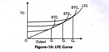
The LTC curve is shown in Figure-10:
As shown in Figure-10, short run total costs curves; STC1, STC2, and STC3 are shown depicting different plant sizes. The LTC curve is made by joining the minimum points of short run total cost curves. Therefore, LTC envelopes the STC curves.
2. Long Run Average Cost:
Long run Average Cost (LAC) is equal to long run total costs divided by the level of output. The derivation of long run average costs is done from the short run average cost curves. In the short run, plant is fixed and each short run curve corresponds to a particular plant. The long run average costs curve is also called planning curve or envelope curve as it helps in making organizational plans for expanding production and achieving minimum cost.
ADVERTISEMENTS:
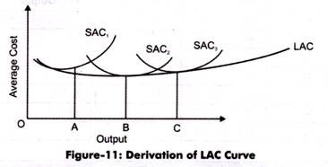
Figure-11 shows the derivation of LAC curve:
Suppose there are three sizes of the plant and no other size of the plant can be built. In short run, the plant sizes are fixed thus, organization increase or decrease the variable factors. However, in the long run, the organization can select among the plants which help in achieving minimum possible cost at a given level of output.
From Figure-11, it can be noted that till OB amount of production, it is beneficial for the organization to operate on the plant SAC2 as it entails lower costs than SAC1. If the plant SAC2 is used for producing OA, then cost incurred would be more. Thus, in the long run, it is clear that the producer would produce till OB on plant SAC2. On SAC2, the producer would produce till OC amount of output. If an organization wants to exceed output from OC, it will be beneficial to produce at SAC3 than SAC2.
ADVERTISEMENTS:
Thus, in the long run, an organization has a choice to use the plant incurring minimum costs at a given output. LAC depicts the lowest possible average cost for producing different levels of output. The LAC curve is derived from joining the lowest minimum costs of the short run average cost curves.
It first falls and then rises, thus it is U- shaped curve. The returns to scale also affect the LTC and LAC. Returns to scale implies a change in output of an organization with a change in inputs. In the long run, the output changes with respect to change in all inputs of production.
In case of increasing returns to scale (IRS), organizations can double the output by using less than twice of inputs. LTC increases less than the increase in the output, thus, LAC falls. In case of constant returns to scale (CRS), organizations can double the output by using inputs twice.
LTC increases proportionately to the output; therefore, LAC becomes constant. On the other hand, in case of decreasing returns to scale (DRS), organizations can double the output by using inputs more than twice. Thus, LTC increases more than the increase in output. As a result, LAC increases.
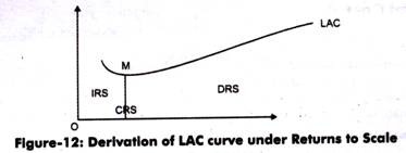
Figure-12 shows the effect on LAC because of returns to scale:
As shown in Figure-12, up to M, LAC slopes downward. This is because at this stage IRS is applied. On the other hand, at M, LAC becomes constant. After M, LAC slopes upwards implying DRS.
3. Long Run Marginal Cost:
Long run Marginal Cost (LMC) is defined as added cost of producing an additional unit of a commodity when all inputs are variable. This cost is derived from short run marginal cost. On the graph, the LMC is derived from the points of tangency between LAC and SAC.
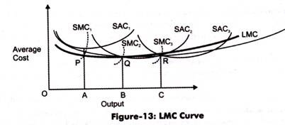
LMC curve can be learned through Figure-13:
If perpendiculars are drawn from point A, B, and C, respectively; then they would intersect SMC curves at P, Q, and R respectively. By joining P, Q, and R, the LMC curve would be drawn. It should be noted that LMC equals to SMC, when LMC is tangent to the LAC.
In Figure-13, OB is the output at which:
SAC2 = SMC2 = LAC = LMC
We can also draw the relation between LMC and LAC as follows:
ADVERTISEMENTS:
When LMC < LAC, LAC falls
When LMC = LAC, LAC is constant
When LMC > LAC, LAC rises


