Theory of Reciprocal Demand (With Criticisms) | Economics

In this article we will discuss about the assumptions and criticisms of the theory of reciprocal demand for commodities.

The Ricardian failure to determine the exact rate of international exchange between the two countries was on account of an excessive emphasis upon the supply aspect and a complete neglect of demand aspect. It was J.S. Mill, who attempted to remove this lacuna in the Ricardian comparative costs theory.

According to him, the actual ratio at which commodities are transacted between two countries depends crucially upon the strength and elasticity of each country’s demand for the product of the other or the reciprocal demand. By reciprocal demand, Mill meant the quantities of exports that a country would offer at different terms of trade, in return of varying quantities of imports. In other words, reciprocal demand refers to the intensity of demand for the product of one country in the other country.

Assumptions of the Theory:

J.S. Mill’s theory of reciprocal demand is based upon the following main assumptions:

(i) The trade takes place between two countries, A and B.

(ii) The trade is in two commodities, X and Y.

(iii) In both the countries, the production is governed by constant return to scale.

(iv) The trade between two countries is governed by the principle of comparative costs.

(v) The pattern of demand is similar in two countries.

(vi) There are perfectly competitive conditions in the market.

(vii) There is no restriction on trade and government follows a policy of laissez faire.

(viii) There is full employment of resources in both the countries.

(ix) There is an absence of transport costs.

(x) The exports of each country are sufficient to pay for its imports.

Given the above simplifying assumptions, Mill’s theory of reciprocal demand can be explained on the basis of Table 5.1.

According to this table, the pre-trade exchange ratio between X and Y commodities in the two countries are:

Country A:

1 unit of X = 0.63 unit of Y

Country B:

1 unit of X = 0.80 units of Y

If trade commences between them, country A specialises in the production of X while B specialises in the production of Y. But the basic issue is concerned with the rate at which they will exchange their goods. The international rate of exchange will be settled within the two limits of domestic exchange ratio on the basis of reciprocal demand or the relative intensity of demand for the products of each other.

If the demand for X commodity is less elastic in country B but the demand for Y commodity in country A is more elastic, the country B will be willing to give more units of Y for importing a given number of units of X and the international rate of exchange will be closer to the domestic exchange ratio of country B. It means the exchange ratio or terms of trade are more favourable to country A and she will obtain a larger share out of the total gain from trade.

On the contrary, if the demand for Y commodity is inelastic in country A and the demand for X commodity is more elastic in country B, the latter will be willing to give up an additional unit of Y in exchange of more units of X commodity. In this case, the international exchange ratio will get settled closer to the domestic exchange ratio of country A. The terms of trade are now more favourable to country B and it will secure a larger proportion of gain from trade.

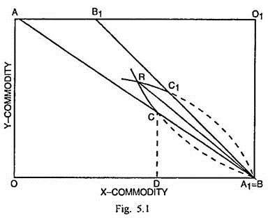
The determination of actual rate of exchange on the strength of reciprocal demand is shown through Fig. 5.1.

AA₁ represents the production possibility curve of country A. It shows the different combinations of X and Y commodities that country A can produce under constant cost conditions and with the fullest utilization of available labour input. Similarly BB₁ represents the production possibility curve of country B with origin as O₁. Suppose country A specialises in commodity X and country B specialises in Y.

If there is complete specialisation, the production point is A₁=B, where country A devotes all productive resources on producing X and country B on producing Y. AA₁ and BB₁ production possibility curves represent also the domestic ratio of exchange. Trade will take place within these two limits. So AA₁B₁ shows the potential trading area. The actual exchange ratio will lie somewhere in this area.

If country A requires OD quantity of X and CD quantity of Y, it can meet the demand through domestic production in the absence of foreign trade. Suppose it requires more quantity of Y than CD. The additional demand for Y can be met by importing it from country B. Now A will offer to give up more quantity of X in order to get additional units of Y. A₁CR represents the offer curve of country A. CA₁ part of this curve is imaginary because all these combinations of X and Y commodities can be obtained through domestic production and without external trade.

Similarly BC₁R is the offer curve of country B and BC₁ part of this curve is imaginary. As we move along CR part of offer curve of country A, the terms of trade become favourable to A. In the same way, the movement along C₁R makes the terms of trade more favourable for B. The two offer curves intersect each other at R.

At this equilibrium position, exports of each country are just sufficient to pay for imports. Any change in reciprocal demand will cause a variation in this actual exchange ratio. The more inelastic the offer curve of the country, the more favourable will be the terms of trade for her and vice-versa. The line joining R and A₁ (or B) denotes the actual exchange ratio of two commodities for the two countries.

Ellsworth and Leith have summed up the theory of reciprocal demand as follows:

“In summary, (1) the possible range of barter terms is given by the respective terms of trade as set by comparative efficiency in each country; (2) within this range, the actual terms depend on each country’s demand for the other country’s produce; and (3) finally, only those barter terms will be stable at which the exports offered by each country just suffice to pay for the imports it desires.”

It is possible to explain J.S. Mill’s theory of reciprocal demand through the use of Marshall’s device of offer curve. The offer curve of a country describes the different quantities of her product that can be offered to the foreign country to meet the demand for certain quantities of the product of the foreign country.

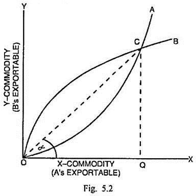
It is the demand for the product of each other or reciprocal demand, on the basis of which the offer curve of each country can be determined. In what way the terms of trade between countries A and B related to two commodities X and Y, can be determined is shown through Fig. 5.2.

In Fig. 5.2, X-commodity which is A’s exportable is measured along the horizontal scale and Y-commodity which is exportable of B is measured along the vertical scale. OA is the offer curve of county A and OB is the offer curve of country B. Every point on curve OA indicates different quantities of X which country A offers in exchange of various quantities of Y.

Similarly the different points on the offer curve OB of country B show the quantities of commodity Y that country B offers for exchanging them with different quantities of X commodity. The equilibrium exchange takes place at C where the two offer curves cut each other. The country A exports OQ quantity of X in exchange of CQ quantity of Y-commodity. The terms of trade (TOT) are measured by the ratio of quantity imported (or demanded) to the quantity exported (or supplied), which in the equilibrium position C is CQ/OQ.

TOT at C = Q_M/Q_X = CQ/OQ = Slope of line OC = Tan ∝

If country A’s demand for product Y increases, she would be willing to offer more quantities of X for the same quantities of Y. In such a situation, the offer curve of country A will shift to the right. On the opposite, if A’s demand for product Y decreases, she would offer less quantities of X in exchange for the same quantities of Y. In this case, the offer curve of country A will shift to the left of its original position.

Similarly, if country B’s demand for X increases, she would be willing to offer more quantities of Y in order to have the same quantities of X. That will cause a shift in the offer curve of country B to the left of its original position. On the opposite, a decrease in the demand for X by it will lead to a shift in its offer curve to the right. The impact of these shifts upon the actual equilibrium exchange ratio or terms of trade can be shown through Figs. 5.3 and 5.4.

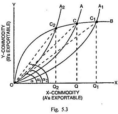
In Fig. 5.3, OA and OB are the original offer curves of the two countries A and B respectively. C is the point of equilibrium exchange and TOT at C = Q_M/Q_X = CQ/OQ = Slope of line OC = Tan ∝. If A’s demand for product Y increases, the offer curve of country A shifts to the right to OA₁. The intersection between OA₁ and OB takes place at C₁, where C₁Q₁ quantity of Y is important in exchange of OQ₁ quantity of X.

The TOT at C₁ = Q_M/Q_X = C₁Q₁/OQ₁ = Slope of line OC₁ = Tan ∝₁. Since Tan ∝₁ Tan, the TOT have become unfavourable for country A or favourable for country B. If A’s demand for product Y decreases, the offer curve of A shifts to the left from OA to OA₂ and exchange equilibrium takes place at C₂ through the intersection of curves OA₂ and OB.

Country A imports C₂Q₂ quantity of Y and exports OQ₂ quantity of X. The TOT at C₂ = Q_M/Q_X = C₂Q₂/OQ₂ = Slope of line OC₂ = Tan ∝₂.

Since Tan ∝₂ > Tan ∝ the terms of trade have become favourable for country A or unfavourable for country B.

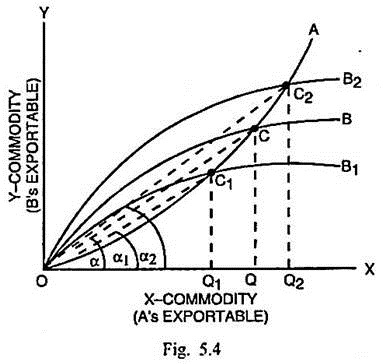
In Fig. 5.4, given OA and OB as the offer curves of countries A and B respectively, C is the point of exchange. Country A exports OQ quantity of X in order to import CQ quantity of Y. The TOT at C = Q_M/Q_X = CQ/OQ = Slope of line OC = Tan ∝. If B’s offer curve shifts to the left to OB₂, where B’s demand for X-commodity increases, the equilibrium takes place at C₂ through the intersection of OA and OB₂. At point C₂, country B imports OQ₂ quantity of X and exports C₂Q₂ quantity of Y commodity. From the point of view of country A, the TOT at point C₂ = Q_M/Q_X = C₂Q₂/O₂Q = Slope of line OC₂ = Tan ∝₂.

Since Tan ∝₂ > Tan, there is improvement in the TOT for this country. It signifies that the terms of trade have gone against the country B. On the opposite, if B’s demand for X-commodity decreases, it offers less quantities of commodity Y for having the same quantities of X as before. In the situation, the offer curve of country B shifts to the right to OB₁. The exchange takes place at C₁ where OB₁ intersects OA. Country B imports OQ₁ quantity of X and exports C₁Q₁ quantity of Y. From the point of view of country A, the TOT at C₁ = Q_M/Q_X = CQ₁/O₁Q = Slope of line OC₁ = Tan ∝₁.

Since Tan ∝₁ < Tan ∝, there is worsening of the terms of trade for country A while these become favourable for country B. Thus the intensity of demand for the product of each other determines the changes in terms of trade for the trading countries.

The actual equilibrium exchange rate is determined also by the elasticity of the offer curves of the trading countries. Greater the elasticity of the offer curve of a country, the more adverse are the terms of trade for it in relation to the other country and vice-versa.

Mill’s theory of reciprocal demand analysed in terms of the offer curves of two countries, can also provide a measure of distribution of gains from trade among the two countries. It can be explained through Fig. 5.5.

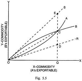
In Fig. 5.5, OA and OB are the offer curves of countries A and B respectively. The slope of the line OR measures the domestic exchange ratio in country A. The slope of line OS measures the domestic exchange ratio of country B. When trade takes place, the exchange equilibrium is determined at C where OA and OB cut each other. The international exchange ratio is measured by CQ/OQ or the slope of line OC.

In the absence of trade, given the domestic exchange ratio line OR, country A exchanges DQ of Y with OQ of X but after trade takes place, she can import CQ quantity of Y in exchange of the export of OQ quantity of X. Thus gain from trade for country A is equivalent to CQ – DQ = CD units of Y.

In the case of country B, the pre-trade position, given the domestic exchange ratio line OS was that she exchanged EQ quantity of Y with OQ quantity of X. But after trade commences, country B exports only CQ quantity of Y for the import of OQ quantity of X. Thus the gain from trade for country B is EQ – CQ = EC. Closer the international exchange ratio line to the domestic exchange ratio line of one country, greater is the gain from trade for the other country and vice-versa.

Criticisms of the Theory of Reciprocal Demand:

The theoretical structure of J.S. Mill’s theory of reciprocal demand rests upon the foundation of Ricardian principle of comparative costs.

Consequently, the theoretical assumptions in Mill’s theory are almost the same as in the Ricardian theory. That makes Mill’s theory of reciprocal demand susceptible to similar weaknesses as are found in the Ricardian analysis.

In addition to structural deficiencies, Mill’s approach has been attacked by F.D. Graham and Jacob Viner on the following main grounds:

(i) Neglect of Supply:

According to Graham, the reciprocal demand theory concentrates too much on demand for determining the international values and the supply aspect has been grossly neglected. Such an approach can be accepted, if the theory of international trade is built in terms of fixed quantities of product. In practice, trade involves such commodities the supply of which undergoes significant variations. Therefore, the supply conditions are bound to have decisive effect on the international exchange ratio.

(ii) Unnecessary:

Graham dismissed the whole idea of reciprocal demand as unnecessary in the theory of international values. If the production takes place under constant cost conditions, as assumed both by Ricardo and Mill, the supply conditions alone are sufficient to settle the final equilibrium rate of exchange.

(iii) Neglect of Domestic Demand:

In this theory, the international exchange is supposed to be influenced by the demand in one country for the product of the other or the reciprocal demand. The domestic demand in each country for her exportable product can also exert an important influence because each country is likely to export the product, which is left after satisfying the domestic demand. The determination of exchange ratio, by overlooking the domestic demand, was clearly faulty.

(iv) Not Relevant in Multi-Country, Multi- Commodity Trade:

The entire analysis in the Ricardian-Mill comparative costs theory is in terms of a two-country and two-commodity model. In the real world multi-country, multi-commodity trade situation, there is strong possibility that the international terms of trade are determined by the cost ratios rather than the reciprocal demand.

(v) Size of Trading Countries:

The reciprocal demand theory can possibly influence the terms of trade between the two trading countries, provided the two countries are of equal size and the values of their respective products are also equal. However, if one of the two countries is large and the other is small, the gain from trade goes largely to the smaller country rather than the larger country.

Since the produce of smaller country is not sufficient to meet the needs of the larger country and at the same time, the former cannot absorb fully the produce of the latter, there will be incomplete specialisation in the larger country but a complete specialisation in the smaller country. The smaller country will have to take whatever is offered by the larger country and export what is required by latter.

In the trade between the countries of unequal size, therefore reciprocal demand has little relevance. A small country is usually a price-taker rather than a price- maker. Since the terms of trade are likely to be close to the domestic exchange ratio of larger country, the major beneficiary from trade would be the smaller country rather than the larger country.

(vi) Variations in Income:

Mill’s theory of reciprocal demand maintains that income levels in two countries remain the same. Such an assumption is unrealistic. In addition the variations in income may have effect upon the terms of trade between the trading countries. This theory tends to overlook the impact of income variations on the terms and pattern of trade.

(vii) Over-Simplification:

The theory of reciprocal demand is an over-simplification of reality. In the determination of international terms of trade, it fails to take into account such significant factors as wage-price rigidities, price movements and balance of payments conditions.

There is no doubt that some of the arguments advanced by Graham do carry some weight. The neglect of supply factor was certainly a serious lapse on the part of J.S.Mill but it is not realistic to suppose that the reciprocal demand has absolutely no significance. In the words of Findlay, “The fact that the terms of trade will usually be equal to the cost ratio of some intermediate or ‘marginal’ country does not mean that demand can be dispensed with, for it is precisely the demand condition that determines which is the marginal country whose cost ratio is equal to the terms of trade.”

In fact, much of Graham’s criticism of reciprocal demand theory was unwarranted and misguided. In the conditions of increasing costs, when the countries are likely to have incomplete specialisation, both cost ratio and reciprocal demand must determine the terms of trade. It is clearly fallacious to dismiss the reciprocal demand as an irrelevant factor in the trade relations among the countries.