General Equilibrium in an Economy | Term Paper | Economics

Here is a term paper on the ‘General Equilibrium in an Economy’ for class 9, 10, 11 and 12. Find paragraphs, long and short term papers on the ‘General Equilibrium in an Economy’ especially written for school and college students.

Term Paper # 1. Introduction to the General Equilibrium in an Economy:

The Walrasian model is an important model of classical economy. The model assumes that there are households and firms which are exchanging goods. Such exchange of goods is depending on the bargaining of the two individuals. Here, households supply services to firms and the firms supply goods to the households resulting in a circular flow in the economy. The prices of commodities are determined on the basis of the market mechanism. There is no scope for individuals to bargain for price.

It is general equilibrium in the competitive economy. General equilibrium analysis seeks to determine equilibrium prices simultaneously in all the markets. But markets do not work efficiently due to monopoly. Sometime monopoly in market leads to inefficiency in resource allocation and mobilization. Therefore role of government is important in market efficiency. Externality exists in production function of a firm. Negative externalities reduce the production of the firm. Again the role of government is important to correct the negative externality and to improve allocation.

Term Paper # 2. Walrasian Equilibrium of a Competitive Economy:

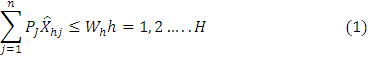
The basic assumption of the Walrasian equilibrium is that the economy is exchange economy. The goods are exchanged for goods in such economy. It has further assumed that there are number of goods produced by firms and consumed by households. Economy consists of households and firms. Firms are producing n goods and households provide services to firms. If we assume that, X̂_hj is the net demand for the j^th good of the h^th household.

Where H = 1, 2,….H . Similarly y_ij the net supply of the good by the i^th firm where i= 1, 2,…M. The supply of goods by firms and demand of goods by households is measured and it is negatively co-related. Household’s strictly quasi-concave utility function is presented as u_h(X̂^h) where X̂^h = (X̂_h1, X̂_h2,…………………… X̂_hn). Each household maximizes the utility subject to the budget constraints. Each household has scare resources and its effect on the budget constraint.

Household’s budget constraint is presented as:

Where

W: Household wealth which is measured in terms of rupees.

Each household owns wealth in the form of physical and financial assets. Financial asset consists of shares, bonds, debentures etc. Firms provide financial investment opportunities to households. Households invest in a given vector of shares in firms. It is = β_h = (β_h1,………. β_hm) with 1 ≥ β_hi > 0 all h, i. We have assumed that ∑_hβ_hi = 1. Profit of the firm is positively co-related to the household’s wealth. Firms provide dividend on the shares owned by the households.

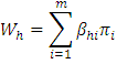
Where π_i is profit of the i^th firm which earned out of production. Household’s financial wealth consists of the sum of its shares owned of firm and dividend paid by firm.

Firms wish to maximize profit from output. Such output is multiplied with price level in market. The sale of output in market provides profit to firm.

It is defined as:

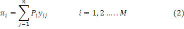
But the profit of a firm is subjected to the production possibilities frontier. Firm produces output after using the inputs.

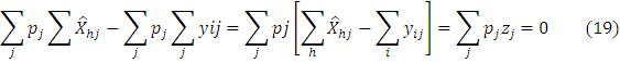
Such output satisfies the following condition:

Where y_i = (y_i1,y_i2,y_in). Output of firm is always greater than zero. Firm’s production function (f_i) exhibits strictly diminishing returns. Diminishing returns of a firm is a long term phenomena. Each firm’s production set is strictly convex.

Firm produces output which is demanded by household. The household’s net demand function is presented as follows-

And each firms net supply function is as follows:

Income to firms is a function of supply of number of commodities to household. The goods consist of p₁ to p_n.

Properties:

(a) The price vector is given for market and there is market mechanism which decides the unique demand and supply. It is uniquely determined in the market for different commodities.

(b) Prices do not change in short term. The net demand and supply varies continuously with prices.

(c) Suppose all prices change along with demand and supply of commodities then the net demand or supply is unchanged.

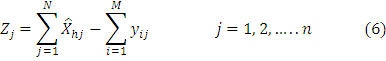
Now we will consider commodity j. The demand and availability of supply of such commodity shows the deficit and excess stock of commodity. It is presented in simple equation form.

We refer to Z_j as the excess demand or deficit for good j. It simply represents the difference between net demand and supply of commodity. It is inversely related when supply X_hi is less. There will be excess supply Z_j. The excess demand or supply of any commodity is written in the equation.

The demand and supply of any commodity may be positive or negative. Such demand and supply curve can be presented in the diagram. They are presented in different form as follows. The demand and supply of commodity shows the equilibrium price level.

Diagram 6.1(a) shows the upward sloping supply curve and downward sloping demand curve. Both are intersecting at point E. Such point is known as equilibrium of demand and supply. It is normal market clearing equilibrium of demand and supply. Equilibrium price of j^th commodity is shown on y axis. On x axis, the quantity demanded is shown. At p, there is no change in price and equilibrium of demand and supply is achieved. Such equilibrium is observed for normal goods. For scarce commodities, prices rise continuously.

Diagram 6.1(b) shows the negative demand and supply. The price of commodity is shown as pj which is below zero. At this point, both demand and supply should increase. It will help to increase the prices to rise.

Diagram 6.1(c) explains that demand exceed supply. The price is shown at P*_j. It is positive price but supply is not exists.

Diagram 6.1(d) shows the negative demand. There is no price exist for commodity. Suppose the commodity is supplied then it will have automatic impact on price. It is automatic adjustment in demand and prices.

The purpose of supplying more goods is to control the prices. But at the same time, it is meaningless to supply the commodities at a cheaper rate. The relative prices may not remain same for long term. If the prices start to rise then people buy more substitutes. It will help to reduce the prices of commodities in the longer term. Therefore price is best parameter to make the market at equilibrium.

For economy as a whole, the general equilibrium price vector is defined as (p*1, p*2 ,…p*n).

The vector of excess demands is explained as (z*1, z*2……….. z*n). The properties are explained as follows:

Properties:

1. Any household’s net demand for commodity is X̂*_hj. Such demand is corresponding to Zj*. This is because of the following form.

For all X̂^h satisfying

The price of commodities and net demand of commodities is equivalent to the wealth of the household. Household cannot demand goods if household’s wealth is low.

2. Each firm supply goods in market. The individual firms demand and supply corresponding to Z^∝_j. Such supply is denoted as y_ij. The supply of goods must satisfy the criteria of minimum price otherwise firm will not supply goods in market. Such supply is shown as,

The y_ij is the standard output of a firm. But firms always produce close to the standard output. Therefore actual supply of output by a firm is y_ij. An actual output maximizes profit of a firm which is subject to the price level p*j in the market. Here we are not considering negative prices of commodities. In market, the price is an equilibrium price and it does not change in short term.

We can write equilibrium price as:

In order to decide the general equilibrium, the price level must be equilibrium in every market. Such equilibrium price decides equilibrium demand and supply. We can write the demand vector as follows.

We can modify the above two equation and write it below as another equation as,

Above equation 8, 9, 10, 12 show a general equilibrium. The prices of different commodities are non-negative and they consist of various sets. Such sets are the demand of households and supply of commodities by firms. The demand and supply set are optimal bundles and they correspond to the prices which firm supply goods and households demand such goods. Therefore there is no positive or negative demand for commodities exists.

Walrasian Equilibrium:

In an economy, we assume that there is excess demand for each commodity. Such excess demand function of the Walarasian equilibrium is explained as,

The demand for particular commodity is continues. It is changing with equal proportion of change in price level. Above equation shows mapping from of set of price vector into the set of excess demand vectors. In the equation (13) mapping for strictly positive prices is continuous and at the same time it is homogenous of degree zero. If we consider the set of prices corresponding with the demand and supply of commodities then they are the set of a vector prices (p₁, p₂, …. p_n).

Such set of vector prices are bounded below the condition that p_j ≥ 0. But such set of vector prices are not bounded above the condition. It is only possible if we apply the fixed point theorem. At this point, we can only apply normalization rule at any price vector. It is price vector (P₁, p₂, p₃) in p. For this rule, there is need of new price vector and it is further written as (p¹₁, p¹₂………… p¹_n).

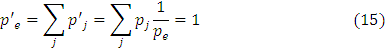
Again by the normalization rule the price vector is written as:

In the equation, e = (I, 1……… 1) and ∑P_j = P_e. It means the cost of a bundle of goods to household. Such bundle of goods consists of one unit of each commodity. The numbers of bundle are written as 1/pe. Such number of bundles can be bought for Rs.10. It is assumed price for a household because it buy number of bundles of commodities.

The normalization rule is helpful to decide the set of normalization price vector p’. In the above equation, such rule is bounded, closed and convex. The price vector P’ is bounded and it is pje”0 for all j. All the price vectors are p’ positive and they are multiplied by (1/p_e) of some p in p and there exist p’j’ ≥ 0 all j. We can now show that p’ is bounded above equation.

It can be represented into following equation: 

We know that the normalization rule for normalized prices is not negative. It means that p¹_j ≤ 1 all j.

We can establish the normal price level as follows:

In the figure 6.2, the normalization procedure is illustrated for n = 2. It shows that the positive quadrant as the set p. Such set of p is corresponding to all pairs of non-negative price vectors (p₁, p₂). In the diagram, the line ab joins the price vectors (0, 1) and (1, 0). Such price vector is the locus of price vectors satisfying the different conditions for n = 2

In terms of equation it is explained as:

Walras’ Law:

The desired net demand vector of household is presented as X̂^h. The planned net supply of firm is shown as the y_i. Household’s net demand X̂^h must satisfy the budget constraints.

Above equation explains that households demand for good is the total demand for j^th commodities. It is equivalent to household’s wealth. The household’s wealth is equivalent to the profit earned by the households from dividend of firm. Therefore,  

Above equation explains that the prices of goods and net demand of households is reduced from prices and output supplied by firm. It is equivalent to the differences between net demand and supply and prices of the commodities. It is further equivalent to the price vector and excess demand for j commodity. Alternatively, at any price vector, the value of the excess demand is exactly zero. Therefore it is marked as zero in above equation. It is known as Walras’ law.

General Equilibrium Proof:

We can explain the excess demand function when the continuity and zero degree homogeneity are given. Such excess demand function is Zj = Zj(p) and pϵp’ . The price vector p* ϵp’ is exist.

We can further explain it as follows:

In the market, there is excess demand and it corresponds to utility maximizing choices by consumers. It is also corresponds to the profit maximizing choices of firms. We can prove the proposition for n goods which are demanded and supplied in the economy.

The proof of such dimension is given as follows:

1. In an economy, the excess demand is defined as continuous function. The mapping from the set of normalized price vector p’ is the set of excess demand vector.

Above equation explains that the excess demand is a function of price level. We can do the mapping of the prices and the net demand.

We need to define the second continuous mapping. It is from the set, where the excess demands back into the set p’. If we take the two compositions of mapping then a continuous mapping of the closed bound convex set is p’. It is a composite mapping which has itself its image. We can do the second mapping which ensures that a fixed point is an equilibrium price vector.

The mapping can be defined by the rule as follows:

Suppose we consider the initial price vector p”p’ and it explains that each corresponding excess demand Z_j(p). The associated price is pj.

A new pj is defined in three ways and after following the rule:

1. We assume that excess demand _Zj(p’) is positive. It adds to the initial price p_j. Some multiple k_j is of the excess demand.

2. Suppose the excess demand for commodity k_j (p’) is zero then the new price observed for the commodity is exactly equal to the old price. Sometimes the commodity price does not change. We observe same price period after period or year after year. Commodities such as biscuits, salt, blades have same prices over the period of time.

3. Suppose old price persists and there is excess demand then the old price p’_j is some multiple K_j of the excess demand unless doing so. It would make the new price negative in which case set instead at zero. We can reapply the normalization rule by summing the prices obtained by applying above rules.

We can define the mapping differently as follows:

In above function, we have presented a continuous function. We need to reconstitute it and therefore composing mapping is defined as-

The above function is also continuous function. It maps the closed bounded convex set p’. Suppose the p’ is given then we can find that z (p’) ϵz. Now we have p = k[z(p’)] ϵ p’

Now, we can apply Brouwer fixed point theorem to prove that there exists a price vector p* ϵ p’ such that-

In terms of equation 22, we can represent the above equation as-

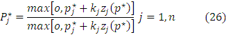
From the above equation, we can prove that p* is an equilibrium price vector. Suppose we assume that the right hand side of above equation is zero then P*_j = 0 for that j. We must have price vector differently and p*_j + k_jz_j(p*) ≤ 0 we must have (since k_j > 0)

If we assume that there are free goods and such goods are either gift of nature or they are provided by government. Therefore the right hand side of the equation is positive and P*_j = 0 for jϵN.

If we multiply through (equation25) by zj (p*) for each jϵ N then we obtain the following equation:

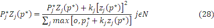
Now we can apply Walras law and rewrite above equation as follows:

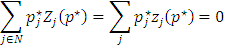
Since P*_j = 0, j∉N, therefore we can sum through (equation 28) over jϵN. It gives us the following equation:

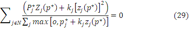
In the above equation, denominator can be cancelled and this is because of some positive number.

By applying the Walara’s law for above equation, we can get the following equation:

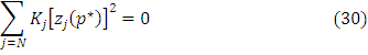
But, since k_j < 0, this can clearly hold only if Z_j(p*) = 0 so

The p* is an equilibrium price vector. It is found in the economy and it provides equilibrium price vector at global level. Since z (p*) is an excess demand vector and it satisfying the requirements (8), (9), p* is non-negative. Therefore equation (10) is satisfied and (11) and (15) together to hold equation (1).

Stability of Walrasian Equilibrium:

In Walrasian equilibrium, stability is an important aspect. The Walrasian equilibrium involves analysis of the movement of prices through successive disequilibrium positions. They are persists over time. In Walrasian equilibrium, there exists at least one equilibrium price vector and it is p* = (p*₁,p*₂,……… p*_n). At an initial movement of time t = 0, there exists a price vector p (0)≠ p*. The time is varying and changing continuously. Therefore the price vector is itself a function of time.

We can represent it as follows,

Above equation explains that price at particular time is itself a function of price at different time. For stability, we need a function of price at different time. For stability, we need a globally equilibrium system which is stable as-

We can represent that there is an equilibrium price vector p (0). It is an equilibrium price vector p*. At such price level, we can allow different adjustment processes. Such adjustments are dynamic in nature. We need to discuss stability relative to a particular adjustment process.

Tatonnement Process:

In an economy, there exists an umpire whose job is to announce a price vector at each different time. For announcing the prices of different commodities, the umpire collects the information. Sometimes prices are too low or too high, therefore umpire decides whether to permit the trading of commodities or not. In modern economy, government often acts like an umpire, whose job is to collect the data of prices of all commodities and allow the trading of commodities. Suppose prices rising very fast then government takes a steps to reduce the prices.

But there are certain rules and umpire acts according to such rules:

1. An umpire announces a new price vector, if the old prices are not at equilibrium level. There is disequilibrium and the demand and supply of commodities do not match each other.

2. Suppose the demand and supply is not equilibrium at equilibrium price then umpire is not permitting the actual trading of commodities.

3. Suppose there is excess demand of commodities and umpire changed a given price say j^th where j = 1, 2 …n. Such price is proportionate to the excess demand for the corresponding j^th commodity.

That is given the prices p_j (t) at time t is announced by the umpire.

It is as follows:

For an equilibrium price vector, the Walras’ law persists. At announced price vector, consumers buy different commodities and get maximum satisfaction. It is budget constraint which satisfies the consumer’s net demand. Such adjustment is continuous and time cannot restrict such adjustments. Walras’ law is aggregating the households and firms. The households are buying many commodities at prevailing price and firms are selling the commodities at existing price level. Suppose there is disequilibrium in either supply or demand then it has reflection on the price level.

At equilibrium trade will take place. Therefore Walras’ law will not observe here. But for global stability, we required the Walras’ law to satisfy the different conditions. With the help of tatonnement process, we can formulate the global stability system.

But due to more number of commodities in the market, the tatonnement process could be exhaustive. In order to decide the global stability system, we required to assume that there are only two goods traded in market. It will help us to provide tatonnement process in complete form. We can assume that there is demand that exist an equilibrium price vector (p* > 0) which is greater than zero.

The excess demand function has the zero degree homogeneity. It helps us to decide the p* which is an equilibrium price vector. It is up* for any u > 0.

Term Paper # 3. Stability Proposition:

In any economy, there are multiple goods produced by firms. But consumer decides to buy particular commodities. But sometimes he/she buy substitutes. The prices of the commodities are decided by tatonnement process.

Such process is explained by the equation as follows:

At particular price vector p(0), the goods market is at equilibrium. Such equilibrium is globally stable for good 1 and good 2.

For good 1 and good 2, there are gross substitutes and they are presented as follows:

In the above example, we have defined two goods and assumed that they are close substitutes. But we do not know which are goods substituted. In order to find the substitutes, the process is difficult and wider. We are deciding the global equilibrium price level with particular demand and supply. Therefore supply of commodities is important rather than demand by consumers. For deciding the stability proposition, we required some propositions.

Such propositions are explained as follows:

1. We have assumed that there are two goods and they are substituted. The equilibrium price vector is unique. For our understanding if it is assumed that there are two price vectors for two commodities then, it is written as P* = (p*₁,p*₂). Such price vector is unique. Suppose, we assume that there are two price vectors and they are at equilibrium. Let’s assume that p* and p** are at equilibrium. Therefore zj(p*) = zj(p**) = 0 all j.

The gross substitutability explains that p** = up*. We have considered that u is some positive number. We have already assumed that p* and p**. At such equilibrium price vectors, there does not exist. This assumption is contradictory with our earlier assumption.

The following diagram show that p* line is 45° line and it is upward slopping. It is named as up* line. Such line shows the set of all price vectors available for consumers. Such price vectors are scalar multiples of p*. This is because the zero degree homogeneity of the excess demand functions. Suppose p* is an equilibrium price vector then up* must be for any u > 0

In figure 6.3, if we assume that p**'”up*, then the line op** must be distinct from op*. Such effect is shown on two separate lines. Suppose the p* is an equilibrium price vector in the diagram then it must be any point on the op** line.

Since such a point of above figure can be written as follows:

Point p̂** in the figure can be compared with the vector p*, we have,  

Now, p* is an equilibrium point as we have pointed in the diagram.

Therefore we must have the following function which is slightly different:

For the above function, we have applied the gross substitutability. Therefore the above two equations (38 and 39) can be written as:

Since p̂** comprises as the lower price of good 2 than p*. Above equation (41) explains that p̂** is not true equilibrium. It is because p** = (1/u) p**. Therefore it cannot become as equilibrium. Hence an equilibrium price vector can only lie along up*.

2. Gross substitutability with Walras’ law explains that p*₁z₁ (p₁, p₂) + p*₂z₂(p₁, p₂) > 0. Such equation is written to show the disequilibrium in price vector. The equilibrium price vector is written as p = (p₁, p₂).

The disequilibrium excess demands may have effect on prices. But the equilibrium prices must be strictly positive.

The property of the equilibrium is explained as follows:

The new price vector is defined as P̂ which is further defined as follows:

Now we can substitute the new price vector. Therefore gross substitutability is defined as follows. We must have,

Above two equations are unique. But if we combine the equation 43 and 44 together then it implies as follows:

In the above equation, each term must be positive. If we further rearrange above equation then we get the following equation as follows:

Suppose we apply the Walras’ law for above equation then the right hand side of the equation is zero. The proposition is proved because of change of direction in equation 43.

3. We have already assumed that price vector p* is an equilibrium price vector. It is possible from the assumption to define a distance function. It is defined as D (P (t) p*).

Such distance function can be proved slightly different way in terms of derivatives as follows:

In the distance function, D is a real number to each price vector p (t). Such distance function is measuring the distance from equilibrium vector p*. Such function is measuring distance from equilibrium vector p*. It is known in tatonnement process. The Walras’ law and the gross substitute assumption are the two functions which have monotonic values through time. But if fall in price level is observed then there is fall in monotonic values or some scalar multiple of it. But it is an equilibrium vector. The time path of the price vector is getting steadily closer to an equilibrium price vector.