General Equilibrium Theory | Welfare Economics

In this article we will discuss about:- 1. Interdependence in the Economy 2. Graphical Treatment of a Simple General Equilibrium Model 3. Static Properties of a General Equilibrium State 4. General Equilibrium of the Production Sector and the Consumption Sector (Under Perfect Competition) 5. Prices of Commodities and Factors 6. Factor Ownership and Income Distribution and Other Details.

Interdependence in the Economy:

In our dealings with the problems of microeconomic theory we mostly make use of a partial equilibrium approach. In such an approach, we concentrate on decision-making in a particular segment of the economy in isolation of the happenings in the other segments, under the ceteris paribus assumption.

For example, we study the decision-making of a firm in respect of the production of its output and simplify our analysis by assuming that the prices of the factors and products and the state of the technology are given.

Also, product markets, where buyers and sellers interact with each other and among them­selves with regard to the prices and the output levels of various commodities, are studied on the basis of the ceteris paribus assumption, and here the relationships between the markets are ignored.

Similarly, demand, supply and price determination in the factor markets are studied on the basis of the ceteris paribus assumption, and here also the relationships be­tween the different factor markets are ignored. That is, each product and factor market is discussed along the line of the Marshallian partial equilibrium approach and independently of each other.

However, actually, the markets for all commodities and all productive factors are interrelated, and the prices in all markets are simultaneously determined. For example, demand for various goods and services depend on the consumers’ tastes and preferences and incomes.

Consumers’ incomes in turn depend on the amount of resources they own and on the factor prices. Factor prices depend on the demand and supply of the various factors. The demand for factors by the firms depends not only on the state of technology but also on the demand for final goods they produce. The demand for the final goods depends on consumers’ income.

In fact, an economic system consists of millions of economic decision-making units who are motivated by self-interest. Each one pursues his own goal and strives for his own equilibrium independently of the others. In traditional economic theory, the goal of the decision-maker is to maximise (or sometimes minimise) something.

The consumer maximises satisfaction subject to the budget constraint, the firm maximises profit subject to the technological constraints, or the production function. A worker determines his supply of labour on the basis of maximising his satisfaction from his labour-leisure indifference-preference pattern.

The problem here is to determine whether a general equilibrium can be achieved out of the millions of independent, self-interest motivated economic decision-makers, especially in view of the fact that all economic units, be they consumers, producers, or suppliers of factors, are interdependent.

General equilibrium theory tries to ascertain whether independent action by each decision-maker leads to a position in which equilibrium is attained by all. A general equilibrium is defined as a state in which all markets and all decision-making units are simultaneously in equilibrium.

That is, a general equilibrium exists if each market is cleared at a positive price, with each consumer maximising his satisfaction and each firm maximising profit.

The examination of how a state of general equilibrium can, if ever, be reached, i.e., how prices are determined simultaneously in all markets, so that there is neither excess demand nor excess supply, while, at the same time, the individual economic units attain their own goals, falls within the scope of the general equilibrium analysis.

The most ambitious general equilibrium model was developed by the French economist Leon Walras (1834-1910). But in the Walrasian system, [since one of the equations has been found to be redundant], the number of independent equations has been one less than the number of unknowns. That is why the absolute level of prices cannot be determined in this model.

General equilibrium theorists have tackled the problem by choosing arbitrarily the price of one commodity as a numeraire (or unit of account) and expressing all other prices in terms of the price of the numeraire. With this device, prices are determined only as ratios—each price is obtained relative to the price of the numeraire.

This indeterminacy can be eliminated by introducing explicitly in the model a money market, in which money is not only the numeraire, but also a medium of exchange and store of wealth.

But even if there is equality between the number of independent equations and the number of unknowns, there is no guarantee that a general equilibrium solution exists. However, some economists—Arrow, Debreu and Hahn, for example have provided general equilibrium solutions under conditional circumstances.

A Graphical Treatment of a Simple General Equilibrium Model:

We shall show here graphically the general equilibrium, of a simple economy where there are only two factors of production (X₁ and X₂), two-commodities (Q₁ and Q₂) and two consumers (I and II). This is known as the 2 x 2 x 2 general equilibrium model.

Throughout this analysis we shall assume the existence of perfect competition, since it has been proved that a general equilibrium solution exists under free competition (given some additional assumptions about the form of the production and demand functions).

Furthermore, we shall deal only with the static properties of general equilibrium, and we shall not discuss here the dynamic process of reaching the state of such an equilibrium.

The Assumptions of the 2 x 2 x 2 Model:

(i) There are two factors of production X₁ and X₂.

These factors are homogeneous and perfectly divisible. In the model, the quantities of these factors are exogenously given.

(ii) Only two commodities Q₁ and Q₂ are produced. Technology is given, i.e., the production functions remain unchanged in our analysis.

(iii) There are two consumers, I and II, in the economy. They have definite ordinal preference- indifference pattern in respect of consumption of the two goods. All sorts of external effects are absent as also advertising and like activities.

(iv) The goal of each consumer is the maximisation of his own satisfaction subject to his income constraints.

(v) The goal of each firm is profit maximisation, subject to the technological constraint of the production function.

(vi) The factors of production are owned by the consumers.

(vii) The factors of production are fully employed, and all incomes received by their owners (i.e., consumers I and II) are spent.

(viii) There is perfect competition in the commodity and factor markets.

In this model, a general equilibrium is reached when (a) the four markets (two commodity markets and two factor markets) are cleared at a set of equilibrium prices, viz., p₁, p₂ and r₁, r₂, and (b) each participant economic agent (two consumers and two firms) is simultaneously in equilibrium.

Therefore, the solution would give us the values of the following variables:

(i) The total quantities, q₁ and q₂, of the two commodities, Q₁ and Q₂, which will be produced by firms and bought by consumers.

(ii) The allocation of the given quantities, x⁰₁and x⁰₂, of the two factors to the production of each commodity, i.e., the values of x₁₁, x₁₂ and x₂₁, x₂₂. Here x_1i is the quantity of X₁ used to produce the ith commodity and x_2i is the quantity of X₂ used to produce the ith commodity.

(iii) The prices of commodities (p₁ and p₂) and of the factors of production (r₁ and r₂).

(iv) The distribution of factor ownership between the two consumers, i.e., the values of x¹₁, x¹₂ and x¹¹₁, x¹¹₂.

The quantities of factors owned by each individual multiplied by their prices define their income distribution and, hence, their budget constraint.

Static Properties of a General Equilibrium State:

There are three static properties of a general equilibrium solution, reached with a free competitive market mechanism. These are:

(a) Efficient allocation of resources among firms (equilibrium of production).

(b) Efficient distribution of the commodities produced between the two consumers (equilibrium of consumption).

(c) Efficient combination of products (simultaneous equilibrium of production and consumption).

The conditions that have to be satisfied for achieving these efficiencies are known as the marginal conditions for Pareto optimality or Pareto efficiency. 

General Equilibrium of the Production Sector and the Consumption Sector (Under Perfect Competition):

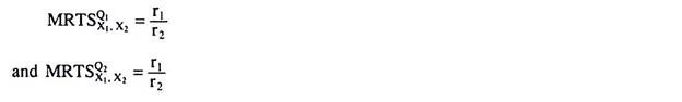
Pareto efficiency in production has given us that the general equilibrium of production occurs at a point where the MRTS between the inputs is the same for all the firms, and this condition is automatically satisfied under perfect competition in the factor markets.

Similarly, Pareto efficiency in exchange (consumption) gives us that the general equilibrium of exchange occurs at a point where the MRS between the goods Q₁ and Q₂ is the same for all the consumers. This condition is also automatically satisfied under perfect competition in the product markets.

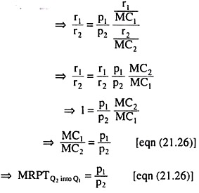
Lastly, Pareto efficiency in product-mix ensures the simultaneous equilibrium of production and consumption and this equilibrium occurs when MRPT of Q₂ into Q₁ becomes equal to MRS of Q₁ for Q₂ of each consumer. This equilibrium is guaranteed when there is perfect competition in the factor and product markets.

We may now briefly describe the steps through which the general equilibrium of the production sector and the consumption sector is established following the principles of Pareto efficiency, provided there is perfect competition in the factor and product markets.

Step I.

Construction of the Edge-worth contract curve for production (CCP) on the basis of the given state of technology, production functions and isoquants (IQs), and the given quantities, x⁰₁ and x⁰₂, of the two inputs, X₁ and X₂.

Step II.

Selection of the point on the CCP, like e in Fig. 21.1, where the numerical slopes of the IQs for the two goods become equal to the numerical slope, r₁/r₂, of the line ST.

At the point e, the efficiency condition (21.1) for production has been satisfied, and, at this point, we obtain the quantities x⁰₁₁, x⁰₁₂ of the two inputs to be used in the production of Q₁ and, x⁰₂₁, x⁰₂₂ the production of Q₂. Also if these input quantities are substituted in the respective production functions, we obtain the output quantities q⁰₁ and q⁰₂ represented by the IQs at the point e.

Step III.

Construction of the production possibility curve or frontier (PPC or PPF) of the economy by means of the mapping of the (q₁, q₂) combinations implicitly obtained at the points on the CCP, in the commodity space of Fig. 21.5.

Each (q₁, q₂) point on the PPC being a (q₁, q₂) combination on the Edgeworth CCP, satisfies the condition:

Step IV.

Finding out the equilibrium point for Pareto-efficient product mix (q⁰₁, q⁰₂). This is given by the point of tangency E between the PPC and the line AB in Fig. 21.5, with numerical slope = p₁/p₂. At the point E, conditions (21.27) and (21.28) are satisfied.

Step V.

Selection of the point e on the Edgeworth contract curve of exchange (CCE) in Fig. 21.5 which has been constructed with q₁ and q₂ as dimensions of the box diagram.

At point e, the numerical slope of the PPC (= p₁/p₂) has been equal to the numerical slopes of the ICs, and so we have:

Fig. 21.1 gives us the allocation of resources at the point of general equilibrium. Of the given quantity x⁰₁ of the input X₁, x⁰₁₁, would be allocated to the production of the commodity Q₁ and x₂₁ would be allocated to the production of Q₂ (x⁰₁₁, + x⁰₂₁ = x⁰₁). Similarly, of the given quantity x⁰₂ of the input X₂, x⁰₂ would be allocated to the production of Q₁ and x₂₂ would be used in the production of Q₂ (x⁰₁₂ + x⁰₂₂ = x⁰₂).

Prices of Commodities and Factors:

We have yet to analyse the determination of the prices in the general equilibrium model. In our simple 2 x 2 x 2 model, there are four prices to be determined. These are the prices, p₁ and p₂, of the two commodities, and the prices, r, and r₂, of the two factors. However, given the assumptions of the simple model, we have three independent relations, i.e., we would have one equation less.

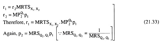
First, profit-maximisation by the individual firms implies least-cost production of the outputs and the conditions for this are:

Since (21.32a) is the same as (21.29), we have here three independent equations in four unknowns. Therefore, the absolute values of r₁, r₂, p₁ and p₂ cannot be uniquely determined although the general equilibrium solution is unique.

Here what we can do is to express the three of the prices in terms of the fourth one, i.e., the fourth price may be taken as a numeraire. For example, let us accept p₁ as a numeraire and express the other three prices in terms of p₁.

We may do the working as follows:

From (21.30)—(21.32), we have:

The above equations give us the relative prices of X₁, X₂ and Q₂ in terms of the numeraire p₁:

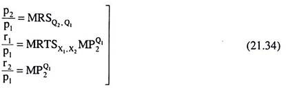
Since the terms on the right hand side of the equations (21.34) are known values which are determined by the general equilibrium solution and the maximising behaviour of the producers and consumers with a given state of technology and given tastes, we have been able to determine the relative prices on their left hand sides.

It may be noted that any good can serve as a numeraire and a change in numeraire would leave the relative prices unaffected. Here the prices are determined as relative prices or as a ratio, because money has not been introduced in the system as a commodity for transactions or as a store of wealth.

The general equilibrium model can be completed by adding one more monetary equation. Then the absolute values of the four prices can be determined in terms of money.

Factor Ownership and Income Distribution:

For the general equilibrium of production and consumption, consumers must earn appropriate incomes so that they may be able to buy the quantities of the two commodities, viz., q⁰₁₁, q⁰₁₂, q⁰₂₁ and q⁰₂₂, implied at the point e of Fig. 21.5.

Consumers’ income depends on the distribution of factor ownership, i.e., the quantities of the factors which they own, and on factor prices. We have already seen that the prices of the factors are determined only as a ratio.

This, however, is adequate for the required income distribution, if the ownership of the factors by consumers I and II is determined. For this purpose, we require four independent relations, given that we have four unknowns, i.e., x^I₁, x^I₂, x^II₁ and x^II₂—these are the factor quantities owned by the two individuals (viz., I and II).

Since the constant returns to scale has been assumed in the model, we can make use of the product exhaustion theorem which gives us that if the inputs are paid at the rate of their respective marginal products (i.e., VMPs), the total factor income would be equal to the total value of the product of the economy, i.e., we would have:

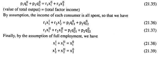
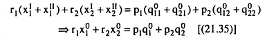
The above five equations, (21.35)—(21.39) give only three independent relations, viz., (21.35), (21.38) and (21.39), because (21.36) and (21.37) are implied by the product exhaustion theorem (21.35):

Thus, here we have three independent equations in four unknowns, whose values, therefore, cannot be uniquely determined. This indeterminacy can be solved partially if we fix up the value of one of the four factor endowments and then determine the remaining three so that the incomes of the consumers would become compatible with their consumption pattern as given at the point e in Fig. 21.5.

It may be noted that the model discussed above assumes that the fixed amounts of the inputs X₁ and X₂ are given. The factor supplies do not depend on the prices of the factors and commodities.

The model could be solved simultaneously for the allocation of inputs, total output-mix and the distribution of commodities, and then only we could superimpose on this solution the ownership of the factors and money income distribution problem.

At the end of this analysis of the simple general equilibrium model, we may conclude that although the model has various shortcomings, it is the most complete existing model of economic behaviour. The students of the subject become aware of the tremendous complexity of the real world as they go through the vast system of mutually interdependent markets.

General Equilibrium and the Allocation of Resources:

The PPC is the locus of points of the Edge-worth contract curve of production (CCP) mapped on the production space [i.e., (q₁, q₂) space], i.e., there is a one-to-one correspondence between the points on the CCP and those on the FPC.

Therefore, we would have a point, say, e in Fig. 21.6 on the CCP corresponding to the point E on the PPC in Fig. 21.5. The production quantities at both E and e are the same, being q⁰₁ and q⁰₂. The allocation of the given quantities of the factors, (x⁰₁₁ and x⁰₂) over the production of the two goods are (x⁰₁₁, x⁰₁₂) for Q₁ and (x⁰₁₁, x⁰₁₂) for Q₂.