Arbitrage Pricing Theory of Portfolio Management | Financial Economics

Capital Assets Pricing Model (CAPM), referred to Arbitrage Pricing Theory (APT) is an equilibrium model of asset pricing but assumes that the returns are generated by a factor model.

Its assumption vis-a-vis those of CAPM are set out first:

APT:

i. Investors do not look at expected returns and standard deviations.

ii. Risk Return Analysis is not the basis. Investors prefer higher wealth/returns to lower wealth.

iii. APT is based on the return generated by factor models.

CAPM:

i. Investors look at the expected returns and ac­companying risks measured by standard devia­tion.

ii. Investors’ are risk averse and risk-return analysis is necessary.

iii. Investors maximise wealth for a given level of risk.

Asset price depends on a single factor, say GNP, or Industrial Production (IP) or inte­rest rates, Money Supply, Inflation rates and so on.

Equation:

Y_i = a_i + bif + e_i; γ_i is expected return from asset i, a_i is the risk free return or constant, f is the value of one of the factors listed above, e_i is the error term (unexplained variables).

A number of variables are taken into account for the Asset price model. This model takes more than one factor, referred to already into the equation say, F_t for interest rate and F₂ for I.P., etc.

γ_i = a_i + b_ilF_l + b_i2 F₂ + e_i we can have F₁, F₂ F₃ etc. in the above equation, a_i is the expected value if all the factors are of zero values (a is constant).

Asset Selection in the Above Model — Sensitivity Analysis:

Investment strategies of many types can also be selected under this model. If there are many securities to be selected, and a fixed amount to be invested, the investor can choose in a manner that he can aim at a zero non-factor risk (ei = 0). This is possible by combining securities to hedge out the sensitivity of a portfolio to all but one factor.

An example will explain this. Let there be three securities A, B and C with the following securities:

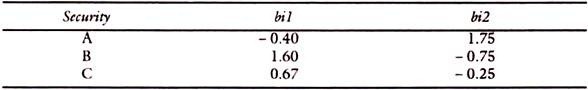
If he has Rs. 1,000, he invests Rs. 300 in Security A, Rs. 700 in Security B and nil in Security C, with proportions being 0.3 in A, 0.7 in B and 0 in C.

It will be seen from the equations below that the sensitivity to factors 1, and 2 will be 1.0 and 0 respectively.

bp₁ = (-0.40 x 0.3) + (1.60 x 0.7) + (0.67 x 0)

= (-0.12) + (1.12) + (0) = + 1.0

bp₂ = (1.75 x 0.3) + (-0.75 x 0.7) + (-0.25 x 0)

= (0.525) + (- 0.525) = 0

In the above fashion, it would be possible theoretically, although not in practice, to create “pure factor” portfolios that are sensitive to only one factor and have insignificant non-factor risk. But in practice, only impure factor portfolios can be created.

Components of Expected Returns:

It is convenient to break up the expected return into two parts:

(i) Risk free rate of return, and

(ii) The rest in the following equation, rf is the risk free return and Yi is the expected premium return per unit of sensitivity to the factor for Portfolio_i.

rp₁ = rf + λ₁

Similarly, the expected return on pure factor 2 portfolio-

rp₂ = rf + λ₂

Thus, the investor by splitting his funds among risk free portfolios and pure factor portfolios, it is possible for him to form a portfolio with almost any sensitivity to each factor. Although theory claims that the non-factor risk can be reduced to zero, it is not possible in real life. Therefore, in practical investment or in portfolio operations, it is better to combine the Capital Asset pricing theory and the APT Model. Most investors prefer no doubt higher levels of expected return and dislike higher levels of risk. The fact is that there is a tradeoff between them, which is not considered by the APT Model. Synthesis of CAPM and APT is therefore more realistic.

Beta coefficients can be used to reflect the risk factors and factor sensitivities can also be taken into account to arrive at the expected returns. Thus, if the returns are generated by two factor model, the Beta coefficient of a security will be related to its sensitiveness to the factors and factor Betas can be taken to reflect the different sensitivities of different factors.

Beta coefficient for a security could be obtained by dividing Cov (r_ir_m) by the variance of the Market Portfolio (σ_M²)

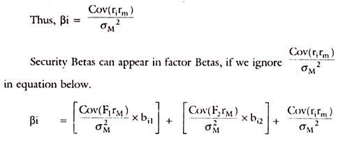
If the last term becomes zero, as referred to above, then-

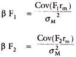
It will be seen that pF, and pF₂ are constants as they do not vary from one security to another, the Beta coefficient of a security is a function of its sensitiveness to the pervasive factors. Thus, by taking Betas of securities the question of sensitivity of security return to a factor is taken care of. By this, one can synthesize the APT Model and CAP Model in the empirical work.

Empirical Testing of APT Model:

The CAPM as also the practical experience tells us that other things being equal, securities with large ex-ante betas will have relatively large expected returns. It does not mean that the actual ex-post returns will also be larger. But investment is made on expectation and hence the use of Betas, despite the fact that exact Betas may not really give an indication of actual returns in future.

Beta measurement is itself subject to limitations, as they change widely, with the number of years for which data are taken, the source of data, and the methods of compilation are subject to normal statistical limitations.

Using the actual data on Stock Price Index numbers and security prices of any Stock Exchange, one can compile Betas. Empirical studies done abroad on NYSE data (by Centre for Research in Security Prices (CRSP) at the University of Chicago) showed that the historical Beta values cannot be counted upon to predict the returns precisely. They are useful as some approximations and landmarks to go by.

In months, in which there were excess positive returns, the Beta factors were generally positive in the sense that stocks with historical Betas gave excess returns over the market. In periods when the excess returns were negative, the Beta factor was generally negative, in the sense that stocks with high historical betas, tended to underperform as compared to those with low historical Betas.

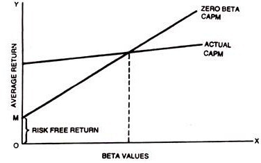
In detailed tests of the original and Zero-beta CAPM, portfolio classes were used to examine the relationship between average returns and historical Betas. The graph below shows the actual relationship for the period 1938 to 1968. The vertical intercept, which corresponds to the zero beta Return, is 0.61% per month, while the average Treasury Bill rate, which corresponds to the risk free rate of interest, was only 0.13% per month. Assuming that Betas are measured relative to a Stock index, they are surrogates for true Betas, and they support the thesis of CAPM to a substantial degree.

In the Graph below, OM is risk free return. Actual CAPM line is shown in the Graph to vary from the Zero Beta line to a substantial extent.