Mundell-Fleming Model | Open Economy | Economics

The Mundell-Fleming model is a model relating to appropriate use of monetary and fiscal policy in an open economy under fixed exchange rates with capital mobility. Under floating exchange rate there is limited scope for government intervention to achieve internal and exter­nal balance. The model differentiates the effect of monetary and fiscal policy on the open economy.

The separation of monetary and fiscal policy was first accomplished by Swan’s model to include capital flows as well. ‘External balance’ or ‘balance of payments equilibrium’ was thus redefined by Mundell to mean a zero balance in the official financing accounts. In the Mundell world, the attainment of the external balance target is influenced by both monetary policy and fiscal policy.

For example, an expansionary monetary policy (in the term of an decrease in the money supply) which reduces interest rates will lead to a reduction in the short- term capital inflows or an increase in short-term capital outflows and to a BOP deficit.

An expansionary fiscal policy—in the term of an increase in income and an increase in imports and also a BOP deficit. Since either expansionary monetary policy or expansionary fiscal policy is assumed to have an adverse effect on the BOP, maintaining BOP equilibrium for a given ex­change rate requires an opposite use of monetary and fiscal policy in this model, i.e., expan­sionary fiscal policy must be supported by centractionary monetary policy, and vice versa.

There is an exactly similar type of policy relationship with respect to the internal balance target. An increase in the money supply leads to lower interest rates and tends to stimulate real investment. This is likely to be expansionary and/or inflationary. So an increase in investment has to be offset by a decrease in government spending or by an increase in taxes that will reduce consumption.

Similarly, maintenance of a given domestic internal balance target indicates that any increase in government spending (or any increase in consumption spending via a decrease in taxes) must be offset by some monetary policy actions such as raising interest rates by reducing the money supply so as to prevent the generation of inflationary pressures within the economy.

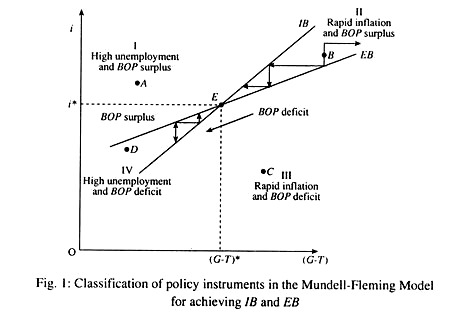
The above policy problem is illustrated in Fig. 1 using a Mundell-Fleming model diagram. On the vertical axis we show the effects of monetary policy through the use of different rates of interest. Fiscal policy is represented through the levels of net government spending (G-T) on the horizontal axis. The inverse relationship between the two policy instruments is shown by the upward sloping curves. Internal balance is represented by the IB curve and the external balance by the EB curve.

In this case, each curve shows combinations of monetary and fiscal policy [i and (G-T)] that bring about internal and external balances. The IB curve is a locus of points showing alternative combinations of interest rate, i (monetary policy) and net government spending (G-T) that ensures internal balance.

Similarly, the flatter EB curve is a locus of points showing alternative combinations of i and (G-T) that ensure BOP equilibrium in the absence of any change in the exchange rate. Points above the IB curve indicate unacceptably high unemployment and points below reflect intolerably rapid inflation.

Similarly, points above the EB curve represent a surplus in the BOP and points below represent a deficit. In Fig. 1, IB and EB are achieved simultaneously at point E which shows a particular combination of i and G-T [i* and (G-T)*].

In Fig. 1, both curves are upward sloping (for reasons already explained). But the EB curve is flatter than the IB curve because changes in the money supply (and, hence, the interest rate) are assumed to have a stronger effect on EB than on IB. This is because changes in the interest rate affect the BOP through both the capital and current accounts.

A change in the interest rate not only leads to a greater net short-term capital inflows but also reduced domestic real investment and income, which act to reduce imports. Changes in the interest rates thus exert both direct and indirect impacts on the BOP, whereas they affect IB only through the direct impact on real investment.

This is known as effective policy classification, which refers to the appropriate assignment of policy instruments to achieve IB and EB simultaneously. In Fig. 1 only one combination of monetary policy and fiscal policy will allow the simultaneous attainment of both targets, that of i* and (G – T)*. If any other combination of the two policies is adopted only one of the two targets, i.e., either IB or EB, can be reached, not both at the same time.

Any point to the left of the IB curve indicates combinations of the two instruments where the interest rate is too high (due to reduced money supply) given the fiscal policy, resulting in low income and unemployment (see point D). Similarly, any point to the right of the IB curve indicates an investment level that is too high, causing demand-pull inflation (such as point C).

Any point to the left of the EB curve shows a rate of interest higher than is necessary to ensure BOP equilibrium at a given exchange rate and, thus, generate a surplus in the BOP due to capital inflows. Any point to the right of the EB curve shows a deficit in BOP because any rate of interest lower than i* leads to outflows of capital. The policy space in the Mundell-Fleming diagram can be divided into four quadrants- each reflecting a different combination of policy targets. See Table 1.

Thus we see that the simultaneous attainment of the two targets is possible only by careful choice of the two instruments involved. For example, if the economy is at point B in quadrant H, expansionary MP is to be used to achieve EB.

A fall in the rate of interest will cause outflow of funds and will thus adversely affect the capital account and, therefore, remove the BOP surplus. At the same time, expansionary FP in the form of a rise in G or a cut in T has to be adopted to achieve IB (high employment without permitting the rate of inflation to accelerate).

An important point has to be noted in this context. It is related to this assignment of instru­ments to targets. Given the nature of IB and EB functions, it will be more efficient to assign the monetary policy instrument to pursue EB and fiscal policy instrument to pursue IB targets. This point becomes clear when we consider the possible sequence of policy steps that could take place at point B.

If monetary policy is used to achieve IB, a decrease in the money supply (or an increase on the interest rate) is called for. If fiscal policy is then adopted to achieve EB, there is need for an expansionary fiscal policy. These steps (shown by the dashed arrow in region II of Fig. 1) would move the economy even further away from i* and (G-T)*, not closer.

On the other hand, using monetary policy to achieve EB and fiscal policy to achieve IB leads to a sequence of policy steps that moves the economy closer to the desired levels i* and (G-T)* (indicated by the leftward pointing arrows in Fig. 1). The same type of policy condition can be reached for points D, C or A.

Thus the Mundell-Fleming model suggests that effective classification of policy instruments and targets is, no doubt, a strategic issue. It is an important element in the successful administration of economic policy in an open economy under fixed exchange rates.

The Assignment Problem:

Let us consider an economy in which the central bank determines the exchange rate (R) and the central government determines fiscal policy. But there is no effective policy coordination between the two authorities. So the question arises as to which agency—the central bank that sets R or the central government that fixes G— should be responsible for EB and which for IB. This question is known as the assignment problem.

If the two instruments are the exchange rate and fiscal policy, the appropriate assignment is to rely on the exchange rate to achieve external balance, and fiscal policy to achieve internal balance.

Whether this is, in fact, the correct assignment depends on the relative impact of the instruments on the two targets:

Target        Instrument:

1. IB Fiscal Policy

2. EB Exchange Rate Policy

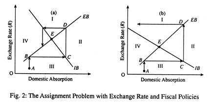
In point (a) of Fig. 2 we show the case where the assignment of the exchange rate to the EB is the correct choice. Suppose the economy starts from points, where there is BOP deficit and unemployment.

Now the central bank decides first to achieve EB. The appropriate devaluation of the cur­rency will move the economy vertically upwards until it is able to reach the EB schedule (see point B). Now there is EB but there is still unemployment at point B. A fiscal expansion will now move the economy to the right until it reaches the IB schedule (see point C).

Now, at point C, the economy has achieved IB, but at the expense of a BOP deficit. A further devaluation moves the economy vertically upwards from point C to D and enables it to reach the EB schedule again. But at point D there is an inflationary pressure.

So the central government has to use a contractionary fiscal policy (reducing G and increasing T) to enable the economy retain the IB schedule and the process continues till point E is reached, at which there is both EB and IB.

In other words, repeated use of the two instruments (exchange rate policy and fiscal policy) will eventually bring the economy at point E at which the EB and IB schedules interact. Thus the adoption of a ‘piecemeal approach’ to policy-making will be con­vergent in nature. (A piecemeal approach to policy-making and policy-implementation refers to adjusting policy in order to attain one policy target and then switching attention to the next policy target and so on).

Part (b) of Fig. 2 shows that the assignment of the exchange rate instrument to the EB target is incorrect. Starting from point A, devaluating to achieve IB and then using an expan­sionary fiscal policy to achieve IB, soon will, in this case, lead to a cyclical movement away from the intersection of the IB and the EB schedules. In this case, the adoption of a piecemeal process will not result in IB and EB simultaneously.

The difference in the two cases occurs due to differences in the slopes of the two sched­ules the relative slopes of IB and EB schedules are different in the two cases. In Fig. 2(a) the exchange rate exerts a much stronger influence on EB than on IB. This means that it would take a greater change in fiscal policy to offset the effects of a currency devaluation on the EB than it would to offset its effects on the IB.

The EB schedule is steeper than the IB schedule. In Fig. 2(b) the exchange rate exerts a relatively stronger effect on the IB. So the IB schedule is steeper. In this case, the correct assignment is to use the exchange rate to achieve IB and fiscal policy to achieve EB.

It was Mundell who first gave us proper guidelines regarding the appropriate assignment of instrument to targets. Mundell’s principle of “effective market classification” states that the policy tools should be assigned responsibility of those policy variables on which they have a relatively stronger influence.

Theory and Practice:

In practice, policy-makers usually take time to enact major policy changes. It is of strategic importance to monitor economic conditions continuously and try to update their policies on a periodic basis. Otherwise, the cure may be worse than the disease, i.e., an effective implemen­tation of a policy may increase the intensity of macroeconomic fluctuations rather than dampen them. Empirical evidence showed that changing the exchange rate had hardly any effect on the BOP but a marked effect on unemployment and inflation.

Further Notes on the Assignment Problem:

Caves and his co-authors have suggested an alternative interpretation of the assignment prob­lem.

In this context they have referred to two policy rules:

Rule 1: Assign EB to the central bank

Assign IB to the central government (or the Treasury)

Rule 2: Assign EB to the central government

Assign IB to the central bank

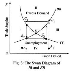
The effectiveness of the two rules depends on the relative slopes of YY and BB schedules, as shown in Fig. 3.

Rule 1 says that whenever there is deficit in BOT, the central bank should devalue (i.e., raise R). Whenever there is a surplus in BOT, the bank should revalue (i.e., lower R). When actual output falls below potential output the government increases G; when actual output exceeds its potential level, the government reduces G.

Let us start from a trade deficit (point A₁). Now the central bank devalues and the deficit is removed (point B₁,). However, a rise in the net exports, under the influence of devaluation, moves the economy into the region of excess demand (and is indicated by a movement from B₁to C₁₎. Now the central government has to reduce G to enable the economy achieve IB at point C₁. However, a reduction in domestic absorption due to cut in G generates a BOT surplus.

Now the central bank has to revalue until BOT surplus disappears at point B₂– However, at point B₂, there is unemployment. So the government has to increase G until the economy re-achieves full employment at G. Once again a trade deficit gives the signal to the central bank to devalue and the process continues until point t is reached, at which IB and EB are achieved simultaneously.

The system is stable here because the YY schedule is steeper (in absolute value) than the BB schedule. If the YY schedule is flatter than the BB schedule the system is unstable, moving further and further away from full equilibrium (i.e., IB and EB at the same time).

Now we apply Rule 2. If there is a deficit in BOT, the government cuts G. Whenever there is a surplus in BOT, the government raises G. IB is assigned to the central bank. Whenever actual output falls below the full employment level, the central bank devalues the currency (raises R); whenever it exceeds the full employment the bank lowers R.

Let us start once again from point A₁. A cut in G leads to unemployment and increase in R and so there is further deviation from point. The system is unstable. There is no convergence. So Rule 2 has failed, since the YY schedule is steeper than the BB schedule. If the BB schedule is steeper than the YY schedule, then the rule will work.

Thus one thing is obvious in this context. The selection of the assignment rule should be based on the relative slopes of two the schedules. The YY line is steeper only if the economy is not very open to imports. In that case, Rule 1 is appropriate fiscal policy and should be used for IB.

By contrast, for a highly open economy, fiscal policy should be assigned to external balance. The reason is not far to seek. If the marginal propensity to import is high, then expenditure-reducing policies are an effective way of improving the BOT—because a high proportion of the reduced expenditure would have been on imports.