Uses of Mundell-Fleming Model in Small Open Economy Case

As students of economics are not supposed to learn but understand the concept, therefore, for better understanding in each topic an appendix is given.

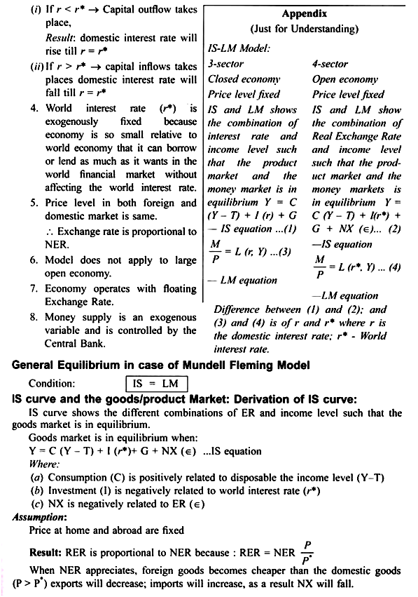
Extension of 3 sector IS-LM model to small open economy (4-sector) under the assumption of perfect capital mobility is called Mundell-Fleming Model.

Mundell-Fleming Model with Floating Exchange Rate and Price Level Fixed:

(Note: In Mundell-Fleming Model as Price level is constant, therefore fixed NER implies fixed RER.)

Mundell-Fleming Model is an extension of three sector IS-LM model to a four sector model, that is, it is a case of a small open economy.

Assumptions:

1. Small open economy

2. Perfect capital mobility

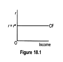
3. Interest rate (r) is determined by the world interest rate (r = r*). CF curve is horizontal parallel to x-axis. It shows that at the world interest rate (r*) it can borrow or lend as much as it wants without affecting the world interest rate.

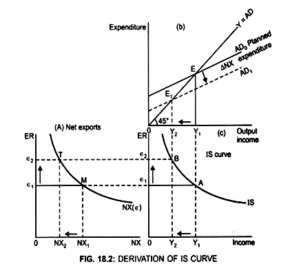
Assume: Initial equilibrium point → M

When RER → є₁ ; NX → NX₁ (Fig, 18.2 (a))

The initial AD curve is AD₀ which intersects 45° line at Income level → Y₁ (Fig. 18.2 (b))

By plotting the combination of Y₁ and є₁ in (Fig. 18.2 (c)) we get first point A on

IS curve

If ER rises from є₁ to є₂

NX falls from NX₁ to NX₂ because ER and NX are negatively related (Fig. 18.2 (a))

As NX is a component of AD

Fall in NX will lead to fall in AD

Therefore, when NX falls to NX₂

AD curve shifts down from AD₀ to AD,

Result:

Income falls from Y₁ to Y₂ (Fig. 18.2 (b))

By plotting the combination of Y₂ and є₂ we get another point B (Fig. C) on IS curve which shows negative relationship between ER and income level.

Thus IS curve in an open economy shows different combinations of ER and income level when goods market is in equilibrium.

Join points A and B the IS curve is derived which is negatively sloped.

LM Curve and the Money Market:

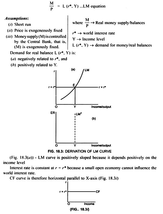
LM curve shows the combination of ER and the income level where the money market clears.

Equilibrium level of income in the money market is determined where:

Supply of real money (M/P) = demand for real balances

Where:

demand for real balance is negatively related to the interest rate (r*) and positively related to income level (Y)

Therefore, LM curve is positively sloped.

As, interest rate is given: r = r*

.^.. Money market is in equilibrium at point E

At point E: Money supply = Money demand

.^.. LM = r* = r at point E (Fig. 18.3(a))

But, as LM is independent of the ER because price level is fixed, therefore, LM curve is vertical straight line (Fig. 18.3(b))

This shows: Whatever be the ER, income level will be determined at the point where LM = r*. This is at point E

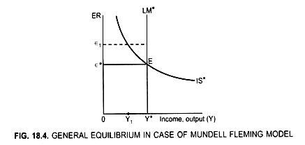
General equilibrium shows the combination of ER and income level where both the goods and money market are in equilibrium.

General Equilibrium in small open economy with perfect capital mobility, according to Mundell Fleming model, is established where

General equilibrium is attained at point E (Fig. 18.4)

This is because at point E, IS^* = LM^*

equilibrium ER → є*

equilibrium income level → OY^*

At any other ER IS ≠ LM

e.g. at ER → є₁ IS^* ≠ LM^*

Money market is in equilibrium at income level → Y^*

Product market is in equilibrium at income level → Y₁

To achieve general equilibrium fiscal or monetary policy is used.