Method of Derivation of the IS and LM Curves (With Diagram)

In this article we will discuss about the method of derivation of the IS and LM curves, explained with the help of suitable diagrams.

(a) Derivation of the IS curve:

The IS curve is frequently derived graphically with a four-part diagram as shown in Fig. 13. Employing simple linear functions, part (a) of Fig. 13 is a plot of the investment function (the MEI); part (c) plots the saving function, part (b) is simply a 45°-identity line; and part (d) plots the commodity market equilibrium, or IS curve.

Picking an initial interest rate level (say, r₀) fixes the level of investment (at I₀) and, thus, the volume of saving (S₀) necessary for equilibrium. Given the volume of saving required, the saving function defines the level of income (Y₀) necessary for equilibrium.

This establishes one point on the IS-LM schedule. Altering the initial interest rate selected by any amount and tracing through the diagram counter-clockwise will yield another point on the IS curve. The resulting IS curve will slope downward from left to right as shown.

The slope depends on two factors, viz.:

(i) Interest-elasticity of investment and

(ii) The numerical value of the multiplier.

(b) Derivation of the LM curve:

Making use of Keynes’ original distinc­tion between transactions and speculative money demands, the LM sched­ule is frequently derived graphically using the four-part diagram. See Fig 14. The schedule in part (b) of the diagram represents transactions demand for money, assuming demand to be proportional (with proportion­ality constant k) to Y.

The schedule in (c) is simply an identity line that mechanically divides the total money supply into transactions and specu­lative components. This part of total money balance (M) not held in one form must be held in the other. The schedule in (a) is the LM curve.

Beginning in (d), with a known interest rate (assume it is r₀), the volume of speculative demand is defined [M _{(spec.) 0}]. Given the total money supply M, that portion not held as speculative balances must be held in transaction balances [M⁰_t] as shown in (c).

The schedule in (b) shows what level of real income (Y₀) must prevail in order to get the public to willingly absorb the money available for transactions balance in that form. Thus, as we see in (a) for interest rate r₀, the only possible money market equilibrium value of income is Y₀.

Should the interest rate rise to r₁, the only possible equilibrium level of income would be Y₁ as we can see by again starting in (d) and proceeding clockwise through our diagram. Thus, the LM curve slopes upward from left to right.

Simultaneous Equilibrium:

By combining the commodity and money market equilibrium schedules (the IS and LM curves) as in Fig. 15, we can see that only one combination of r and Y (the combination r₀ and Y₀) can simultaneously clear both the money and commodity markets.

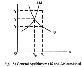
That is, given the money supply and demand schedules that underlay the LM curve, and the consumption and investment schedules that un­derlie the IS curve, the only pos­sible equilibrium values of r and Y are the combination at the IS- LM intersection.

At any other combination of an interest rate and an income level the com­modity market or the money market, or both markets, will be in disequilibrium. If, for example, the level of income should rise (say to Y₁), the rate of interest determined in the money market (r₁) would exceed the interest rate that is necessary (r₂) to stimulate sufficient investment to make Y₁ the equilibrium level of income in the commodity market.

With excess supply in the commodity market, income would be forced downward. If income should ever fall below Y₀, the money market interest rate would fall below the level that would restrict investment to a volume small enough to produce equilibrium in the commodity market. That is, planned investment would exceed planned saving and income would rise.