Wage Determination (With Formula) | Economics

We shall discuss wage determination under imperfect competition with the help of four models of market imperfections.

1.The First Model: Monopoly in the Product Market and Competition in the factor Market—the Monopolistic Exploitation of Labour:

In the first model, we will assume that the firms have monopolistic powers in their respec­tive product markets while the labour market is perfectly competitive.

In this model, monopolistic powers in the product markets imply that, for each individual firm, MR is less than price at all levels of output. Under these conditions, the firm’s MRP_L curve is not the same as its VMP_L curve.

For in this case, we would have:

MRP_L = MP_Lx MR < MP_L x p = VMP_L [MR< p]

i.e., MRP_L< VMP_L                                                 (16.1)

That is, in this case, the MRP_L curve of each firm will lie to the left of its VMP_L curve. However, both these curves owe their shapes to the law of variable proportions.

In this case, as we know, the firm’s demand for la­bour curve would be that part of the negatively sloped portion of its MRP_L curve which lies below its ARP_L curve.

If the firm uses other variable factors also along with labour, its demand curve for labour would consist of the points of shifting MRP_L curves, and this curve also would be negatively sloped.

The market demand curve for labour here is simply the horizon­tal summation of the labour demand curves thus obtained of individual monopolistic firms.

Let us now come to the aggregate supply curve of labour, although there is a general agreement that the supply curve of labour of an individual worker may exhibit the backward bending pattern, it seems that a positively sloped aggregate supply curve of labour is the general case even for the affluent nations.

Higher wages may induce some people to work less hours, but will also attract new workers in the market in the long run.

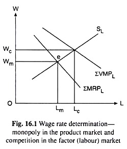
The market price of labour or the rate of wage is determined by the intersection of the market demand and market supply curves for labour, viz., IMRP_L and S_L, as shown in Fig. 16.1 at the point e where the wage rate has been obtained to be W_m. As we have seen, under monopoly, the market demand for labour is based on MRP_L and not on VMP_L.

Only when there is perfect competition in the product market, the market demand is assumed to be based also on VMP_L, because then VMP_L = MRP_L. We have also seen that when the firms have monopolistic powers, labour is paid at the rate of MRP_L, which is less than VMP_L (= W_c).

This effect has been called monopolistic exploitation of labour by Joan Robinson. In Fig. 16.1, this exploitation is given by W_c – W_m, which is the difference between the rate of wage obtained under competition on the basis of VMP_L and that obtained under monopoly on the basis of MRP_L.

2. The Second Model: Monopoly in the Product Market and Monopsony (Single Buyer) in the Labour Market—the Monopsonistic Exploitation of Labour:

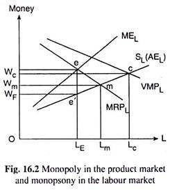
Let us now discuss, with the help of Fig. 16.2, the second model of wage determination under market imperfections, where the firm has monopolistic powers in the product market and monopsonistic powers in the factor market. Here the labour demand curve of the firm is the MRP_L curve (assuming labour to be the only variable factor used by the firm). Also, here the supply curve of labour has a positive slope.

Here, since the firm is the only buyer of labour, it would have to pay a higher wage whenever it wishes to have a larger supply of labour, i.e., it would have to attract labour by paying a higher wage. In other words, the labour supply curve under monopsony would be sloping upward towards right like the curve S_L in Fig. 16.2.

This curve shows the rate of wage or the average expense for labour (AE_L) at different levels of employment. Also, because of the average- marginal relation, the marginal expense for labour (ME_L) curve here would be sloping upwards, and it would lie above the S_L or AE_L curve.

The firm is in equilibrium at L = L_E, when it equates ME_L to MRP_L at the point e in Fig. 16.2. The wage rate that the firm would pay for the L_E units of labour is W_F, which is the equilibrium rate of wage.

When the firm has monopsonistic power in the labour market, it pays to the factor (labour) at a price which is less than not only its VMP but also less than its MRP. This gives rise to monopsonistic exploitation of labour, which is something in addition to the monopolistic exploitation.

Monopolistic and Monopsonistic Exploitation Compared:

We may illustrate the concepts of monopolistic and monopsonistic exploitation and the difference between them with the help of Fig. 16.2.

For the sake of simple illustration we shall use the same set of curves in Fig. 16.2 to represent the market organisations of:

(i) Perfect competition in both product and factor (labour) markets,

(ii) Monopoly in the product market and perfect competition in the labour market and

(iii) Monopoly in the product market and monopsony in the labour market.

In the first case of perfect competition in both the markets, let us suppose that the VMP_L curve is the aggregate demand curve for labour and S_L is the aggregate supply curve. The labour market equilibrium here is obtained at the point c(W_c, L_c). Evidently, here, the rate of wage W = W_c has been equal to VMP_L and so there is no exploitation of labour under perfect competition.

Let us now come to the second case. Here, the MRP_L curve is the aggregate demand curve for labour and the S_L curve is the aggregate supply curve. The labour market equilibrium here is obtained at the point of intersection, m(W_m, L_m) between these curves.

Here, since the rate of wage W = W_m is less than W = W_c, there is labour market exploitation which is called the mo­nopolistic exploitation which amounts to W_c – W_m. Because of monopolistic exploitation, fewer units of labour (L_m < L_c) are used at a lower price per unit (W_m < W_c). However, each unit of input receives an amount equal to what its employment adds to total receipts on the margin.

Lastly, in the third case of monopoly-monopsony the MRP_L curve is the demand curve for labour of the monopsonist buyer of labour and S_L is the supply curve of labour. In this case, the labour market equilibrium will be obtained at the MRP_L= ME_L point e(L = L_E) and here the W – L combination would be obtained at the point e'(W_F, L_E).

Here the rate of wage W = W_F and the employment level L = L_E are not only lower than W_c = VMP_L and L = L_c, but they are also lower than W_m = MRP_L and L = L_m. By definition, the difference between W_c = VMP_L and W_F, i.e., W_c – W_F in Fig. 16.2, is the amount of monopsonistic exploitation of labour, which is as we have already said, something in addition to the monopolistic exploitation of labour.

The W_c – W_m portion of monopsonistic exploitation is attributable to monopoly in the commodity market—it is not unique to monopsony. The additional portion, viz., W_m – W_F, is uniquely attributable to monopsony.

This portion emerges from the fact that each unit of labour employed (barring the marginal unit) receives less than what it contributes to the total receipts (W_F < MRP_L). Thus the monopsonistic exploitation of labour is characterised by the fact that each unit of an input (barring the marginal unit) does not receive as wage an amount equal to its contribution to total receipts.

3. The Third Model: Bilateral Monopoly in the Labour Market:

In the third model of wage determination under imperfect competition, we assume that all the firms are organised in a single body which acts like a monopsonist buyer in the labour market, while the labour is organised in a labour union which acts like a monopolist seller in the labour market.

That is, here we have a case of bilateral monopoly. We shall see here that the solution to a bilateral mo­nopoly situation is indeterminate.

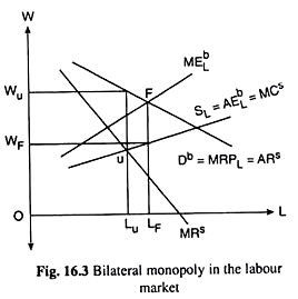
In Fig. 16.3, the monopolist’s (single buyer’s) demand curve for labour is D^b, which is actually the MRP_L curve. From the point of view of the monopolist (the single seller), this curve represents his average revenue (obtained from sale of each unit of labour). So we denote this curve as D^b = AR^S (average revenue of the seller). The seller’s MR^S curve can be derived by using the usual average-marginal relation.

The supply of labour facing the monopsonist is the upward sloping curve S_L = AE^b_L. Corre­sponding to this AE_L curve of the buyer, the marginal curve is ME^b_L.

From the point of view of the monopolist, the curve S_L is its MC curve. If it is assumed that the monopolist behaves as if his prices were determined by forces outside his control, then the MC^S curve may be considered as his supply curve.

Given the above cost and revenue curves, the monopsonist maximises his profit at point F, where his ME_L is equal to MRP_L. Thus, the monopsonist will be willing to hire L_F units of labour and pay a wage rate equal to W_F. The monopolist seller of labour, on the other hand, maximises his profit at point u, where his MC is equal to MR. Thus, the monopolist wants to supply L_u units of labour and receive a wage equal to W_u.

Since the price-goals of the two monopolists cannot be realised here, the price and quantity in the bilateral monopoly market are indeterminate. The only result is the determination of the upper and lower limits (viz., W_u and W_F) to the price. The level at which the price will be settled depends on the bargaining skills and powers of the participants.

4. The Fourth Model: The Firms have No Monopolistic or Monopsonistic Power and the Labour Force is Unionized:

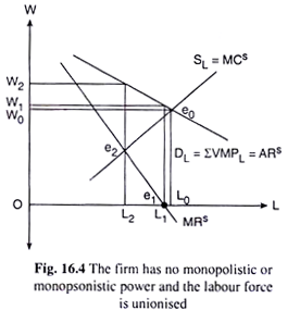
In our fourth and last model, we shall assume that the firms have no monopolistic or monop­sonistic power. The labour force, however, is unionized and behaves like a monopolist seller of la­bour. The situation is shown in Fig. 16.4.

Here the S_L curve shows the MC of the monopolist seller of labour. The market demand curve, D_L for labour, is the aggregate VMP_L curve (IVMP_L) derived from the summation of the individual firms’ demand curves. This curve is also the AR curve of the monopolist seller (union) of labour, from which the MR curve of the seller, MR^s, is derived with the usual method.

The wage in this model depends on the goal of the union. Here we shall examine three of the most commonly pursued goals of labour unions:

(i) The Maximisation of Employment:

The highest level of employment is defined by the in­tersection of the demand and supply curves for labour. Thus, the union will demand a wage rate equal to W₀ in Fig. 16.4. The firms, being price-takers, will maximise their profit by equating W to VMP_L at the point e₀. Thus, the total employment will be L₀.

(ii) The Maximisation of the Total Wage Bill:

If the union aims at the maximisation of total wage bill, it must seek to set the wage at the level at which the marginal revenue (to the union), MR^S, is zero. In this case, the equilibrium of the union is at the point e₁ in Fig. 16.4. The union will set a wage equal to W) and the level of employment will be L₁.

(iii) The Maximisation of Total Gains to the Union as a Whole:

The attainment of this goal requires the union to set the wage at the level corresponding to the equality of MC and MR for the union. The equilibrium of the union is at point e₂ where the wage rate will be W₂ and the level of employment L₂.

Thus, we have seen that the price of an input under imperfect competition in the commodity and the factor markets is determined by the same mechanism as in the case of perfectly com­petitive markets, i.e., demand and supply determine the price of the factor and the level of its employment. However, the determinants of demand and supply are different in the case of market imperfections.