Demand for Complementary and Substitute Goods (Explained With Diagram)

Edge-worth-Pareto Definition of Complementary and Substitute Goods:

Marshall did not give any definitions of substitute and complementary goods.

However before Marshall, Edge-worth and Pareto had provided the definitions of substitute and complementary goods in terms of marginal utility.

According to Edge-worth-Pareto definition “Y is a complementary with X in the consumer’s budget if an increase in the supply of X (Y constant) raises the marginal utility of Y; Y is competitive with X (or is a substitute for X) if an increase in the supply of X (Y constant) lowers the marginal utility of Y.

According to the above Edge-worth-Pareto definition, complementary and substitution relations are reversible, that is, if good Y is complementary with X, X is complementary with Y; and if Y is substitute for X, X is substitute for Y Secondly, assuming that marginal utility of money remains constant, from the above definition it follows that if the price of good X talis and consequently the quantity demanded of good X increases, this will bring about an increase in the marginal utility of good Y if goods X and Y are complementary, and will therefore raise the demand for Y.

On the contrary, if goods X and Yare substitutes, according to Edge-worth- Pareto definition, the fall in the price of good X and consequently the increase in the quantity demanded of X will lower the marginal utility of Y and thereby bring about a decline in the demand for Y. Thus, it is in this way that Edge-worth and Pareto explained the demand for inter-related goods complementary and substitute goods.

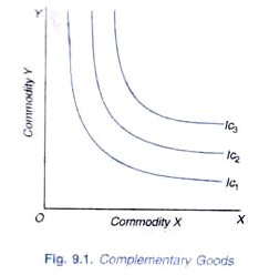
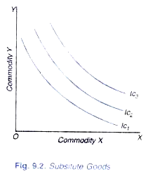
However, Pareto encountered difficulties when he tried to express his definitions of complementary and substitute goods in terms of indifference curves. He opined that the indifference curves between the two complementary goods (according to the above definition) are very bent, as shown in Fig. 9.1 and the indifference curves between two substitutes (according to the above definition) are very flat as shown in Figure 9.2.

Thus Pareto traced parallelism between the complementary goods and the “very bent” shape indifference curves; and between substitutes and very flat indifference curves. But while the definitions make clear cut distinction between complementary and substitute goods, their translation into indifference curves makes the distinction vague, inexact, and imprecise.

This is because the difference between the indifference curves diagrams in Figures 9.1 and 9.2 is not one of kind but of degree. These two diagrams differ only in the curvature of indifference curves; indifference curves in Figure 9.1 have greater curvature than those of Figure 9.2. Now, the pertinent question is what degree of curvature marks the dividing line between substitutes and complementary goods.

Therefore, criticizing Pareto’s aforesaid parallelism Hicks remarks, “the parallelism is not at all exact, as is made evident at once by the impossibility of discovering what degree of curvature of the indifference curves corresponds to the distinction between complementary and substitute goods—which ought, on the above definition, to be a perfectly clear-cut distinction.

Further, the above Edge-worth-Pareto definition of complementary and substitute goods is based on the assumption that utility is measurable. But Pareto regarded the utility to be immeasurable in cardinal or quantitative sense. Therefore, Pareto contradicted himself by defining complementary and substitute goods in terms of measurable utility.

Thus, according to Hicks, “Edge-worth-Pareto definition errs against Pareto’s own principle of the immeasurability of utility. If utility is not a quantity, but only an index of the consumer’s scale of preferences, his definition of complementary goods has a precise meaning. The distinction between complementary and competitive goods will differ according to the arbitrary measure of utility which is adopted.

Hicksian Explanation of Complementary and Substitute Goods:

With indifference curve analysis of demand in which price effect was bifurcated into substitution effect and income effect, Hicks was able to explain in a satisfactory way the cases of substitute and complementary goods. Before Hicks, substitutes and complementary goods were generally explained in terms of total price effect (or in other words, with the concept of cross elasticity of demand).

According to this total price-effect approach, if the price of a good X falls and as a result the quantity demanded of good X increases, the quantity demanded of good Y decreases, then Y is a substitute for X. On the other hand, Y is a complement of X, if with the fall in price of X and resultant increase in quantity demanded of X, the quantity demanded of Y also increases.

Now, according to Hicks, if income effect is taken into account, then even if with the fall in price of X, the quantity demanded of good Y may also increase even though the good Y may be substitute or competitive good. This is when with the fall in price of good there is a large income effect which more than offsets the substitution effect.

Income effect of the fall in price of good X tends to increase the quantity demanded of good Y (as also of the good X) and the substitution effect of the fall in price of X works in favour of X (that is, tends to increase its quantity demanded) and against good Y (that is, tends to reduce its quantity demanded). When this income effect for Y is stronger than substitution effect, then the quantity demanded of Y increases as a result of the fall in price of X, even though the two may be substitute goods.

Therefore, when the income effect is strong enough to swamp the substitution effect for the commodity Y which has become relatively dearer due to the fall in price of good X, the purchases of both goods X and Y increase as a result of the fall in price of good X Then, on the basis of total price effect, the goods would be described as complements, even though they are in fact substitute goods.

Therefore, according to Hicks, goods can be classified as substitutes or complements more accurately by reference to the substitution effect or preference function alone. Hence, in the opinion of Hicks, we can define substitute and complementary goods correctly and precisely only in a situation when we have eliminated the income effect of the price change by making a compensating variation in income. When with a change in price compensating variation in income is also made, the effect which remains is the substitution effect.

Since indifference curve analysis splits up the price effect into income and substitution effects, it is greatly helpful in analyzing the relations of substitution and Complementarity. Take two goods X and Y. If the price of good X falls, price of Y remaining constant, the quantity demanded of good X will increase due to the substitution effect and income effect (we suppose that good X is not an inferior good).

Now, if after the income of the consumer is reduced by compensating variation in income so that with reduced price of good X he is no better off than before, the quantity demanded of X increases and the quantity demanded of Y declines, then good Y is a substitute for X. In this case, due to the relative fall in its price, good X has been substituted for good Y and because of compensating variation in income consumer is no better off than before.

Now, if the price of good X falls and after making compensating variation in income, the quantity demanded of X increases due to the substitution effect and if with it the quantity demanded of Y also increases, then Y is a complement of X Thus, in this case of complements, the quantity purchased of both the goods increases and both of them substitute some other good. Consumer is no better off than before, since compensating variation in income having been made the quantities purchased of two complementary goods has increased due to the substitution effect alone.

In view of the above analysis, Prof. Hicks defines the substitutes and complements in the following way:

“I shall say. Y is a substitute of X if a fall in the price of X leads to a fall in the consumption of Y; Y is a complement of X if a fall in the price of X leads to a rise in the consumption of Y; a compensating variation in income being made, of course in each case. Thus a fall in the price or X, combined with a compensated, variation in income, which must tend to increase the consumption of X itself (by the first substitution theorem), will increase the consumption of complements, but diminish the consumption of substitutes.”

We have seen abovethat the relation of substitutability or complementarity depends on the substitution effect. To determine the substitution effect is quite simple if there are only two commodities on which the consumer has to spend his money income. We know that a fall in the price of good X always leads to the substitution of X for the other goods; and if Y was the only other good available to the consumer, then the substitution effect of the fall in price of good X must necessarily reduce the quantity demanded of Y.

However, when there are more than two goods, a fall in the price of good X may not reduce the quantity demanded of Y; it may in fact increase the quantity purchased of good Y, if the two goods X and Y happen to be complements. Here, the two goods X and Y are substituted for some other goods.

From the above description, it is clear that the definition and proper analysis of substitutes and complementary goods require three goods. That is why J. R. Hicks in his Value and Capital defined them by taking three commodities, X, Y and money and in terms of the concept of marginal rate of substitution. It should be remembered that money stands for all other goods lumped together and is known as composite commodity.

Hicks defined substitute and complementary goods in his book “Value and Capital” in the following way:

“Y is a substitute for X if the marginal rate of substitution of Y for money is diminished when X is substituted for money in such a way as to leave the consumer no better off than before.”

“Y is complementary with X if the marginal rate of substitution of Y for money is increased when X is substituted for money in such a way as to leave the consumer no better off than before.

In order to understand the above definitions, let us assume that a consumer is in equilibrium between X, Y and money so that marginal rates of substitution between them is equal to their respective prices. Now suppose that the price of X falls, prices of Y and money remain the same (price of money is unity). With the fall in price of X, consumer will substitute X for money so that the quantity of X increases and that of money decreases; X is substituted for money.

This will disturb the equality of marginal rate of substitution between Y and money, price of Y being constant. With this, if the marginal rate of substitution of Y for money declines, the consumer must reduce his consumption of Y (that is, he either substitutes X or money for Y) so that the consumer’s marginal rate of substitution of Y for money rises to the level of the unchanged price ratio between Y and money. Therefore, in this case, good Y would be substitute for X since fall in the price of X and consequent increase in its quantity demanded leads to the fall in quantity of Y.

On the other hand, if price of X falls, and consumer substitutes X for money, and as a result of this, the marginal rate of substitution of Y for money increases, consumer will increase the consumption of Y (he will substitute Y for money) so that consumer’s marginal rate of substitution of Y for money falls to the unchanged price ratio between money and Y. Therefore, in this case, Y would be complementary with X since the fall in the price of X and consequent increase in its quantity demanded has led to the increase in quantity demanded of Y.

We thus see that whereas the case of substitutes can be depicted and analysed on a two-dimensional indifference curves diagram, the case of complementarity cannot be done so. This is because in case of analyzing the relation between two complementary goods, at least one other good must be brought into the picture against whom substitution of two complements takes place.

So the case of complementarity cannot arise on a two-dimensional indifference curve diagram. In indifference curve analysis, the case of two complementary goods is generally shown by right angled indifference curves which show that two goods are used in a given fixed proportion. However, the right-angled indifference curves do not indicate the true nature of complements.

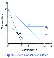
When the price of one complement falls and compensating variation in income is made, the quantities of two complementary goods remain the same, that is, the substitution effect between them is zero, as is shown in Figure 9.3 where as result of the fall in price of good X, the price line shifts from PL₁ to PL₂ and the consumer shifts from equilibrium position Q to Q’.

Line AB is drawn to bring about compensating variation in income (PA in terms of Y is the compensating variation in income). It will be seen from the figure that the price line AB is tangent to the indifference curve IC₁ at the same point Q at which he was in equilibrium before the fail in price of X. Hence, the substitution effect is zero.

However, as we have seen above, in case of two complementary goods, substitution effect between them is not only zero but when the quantity purchased of one good rises due to the compensated price falls, the quantity purchased of the other good also increases. And both these goods substitute some other good.

Further, for the consumer to be indifferent (or no better off) between the two situations, when the quantities purchased of two complements increase as a result of the compensated price fall of one of them, the quantity purchased of some other good must decline against which the two complements are substituted. Therefore, the case of complementarity can arise when there are more than two goods at least three goods among which two are complements and one their substitute.

It follows from the above analysis that while substitutes can occur in case of only two goods, complementary goods cannot be so. When there are only two goods on which the consumer has to spend his income, substitution effect always works in favour of the good whose price has fallen and against the other (that is, it tends to increase the quantity purchased of one and tends to reduce the quantity purchased of the other.)

Thus, if there were only two goods on which the consumer had to spend his income, they would necessarily be substitute goods. Thus case of complementarity can arise only if there are at least three goods. To quote J R Hicks, “If consumer is dividing his income between purchases of two goods only and cannot possible buy any goods other than these two, then there cannot be anything else but a substitution relation between the two goods. For if he is to get more of one of them and still be no better off than before, he must have less of the other. But when he is dividing his income between more than two goods, other kinds of relation become possible.”

Likewise, Prof Hicks writes in his later book “A Revision of Demand Theory”: “If income is being spent upon two goods only, it is impossible that these two goods should be complements. A fall in the price of X must tend to increase the consumption of X (by the first substitution theorem); if it increases the consumption of Y and there are no other goods in the budget, the consumer will have moved to a position in which case he has more Y and no less X; by the consistency theory this cannot be indifferent with his initial position. Thus in the two goods case, the relation between the two goods must be that of substitution; a compensated price change, if it has any effect at all, must lead to more consumption of one good and less of the other.”

Another significant point to be noted regarding the relations of substitutability that whereas all goods in a consumer’s budget can be substitutes for each other, all cannot be complements. Suppose the price of good X falls and consumer’s money income is reduced by the compensating variation in income so as to wipe out the income effect. As a result of this compensated price fall, the quantity purchased of some other goods will decline, that is, good X will be substituted for some other goods.

These ‘some other goods’ whose consumption declines as a result of the compensated price fall of X, are substitutes for X. It is possible that the quantity purchased of some of the other goods may increase as a result of this compensated price fall of X and these would be the complements of X. But while it is possible that all other goods may be substitutes of X, all other goods cannot be complements of X; at least one of the other good must be substitute of X so that substitution of X for it may be done.

To quote J. R. Hicks again, “It is still possible that all other goods may be simply substitutes for one of the goods (say X). This will happen if, when the supply of X is increased, there has to be reduction in the quantities of all other goods. Here the substitution in favour of X is a substitution against each of the other commodities taken separately. But it is possible that there must be an increase in some of the other commodities—commodities complementary with X since the consumer cannot get more of all commodities and still be left no better off than before.”

Compensated Demand Curve:

The ordinary demand curve for a consumer which we derived from the price consumption curve includes the effect of both the substitution and income effects of the changes in price of a good on its quantity purchased. As a consumer moves downward along the ordinary demand curve, he goes to a higher indifference curve on the price consumption curve and his satisfaction or real income increases. It may be noted that in deriving ordinary demand curve, money income of the consumer is held constant.

However, for certain problems such as measurement of consumer surplus, the use of ordinary demand curve is not appropriate. This is because for the proper analysis of consumer surplus we need a demand curve that is based on the real income (i.e., satisfaction) being held constant as price of a good changes rather than money income being kept constant.

Such demand curve which incorporates the effects of changes in price of a commodity, real income remaining constant is called income compensated demand curve or simply compensated demand curve. In the derivation of compensated demand curve, following the changes in price of the commodity, real income is held constant by making appropriate compensating variation in income.

Thus, whereas ordinary demand curve describes the effects of both the substitution and income effects of the changes in price of a commodity, compensated demand curve includes the effect of only substitution effect.

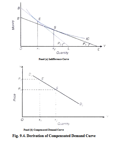
How a compensated demand curve is derived is illustrated in Fig. 9.4. In the upper panel (a) the consumer has money income equal to OB. With initial price of the commodity equal to P₀, (slope of OB/OL = P₀) budget line is BL which is tangent to the indifference curve IC at point E where consumer is buying Ox₁ quantity of the commodity. Now, suppose price of a commodity X falls to price P₁, (P₁= slope of budget line B’L’ = OB/OL) and together with this fall in price, consumer’s income is reduced so that the budget line representing the lower price of X is again tangent to indifference curve IC, although at a different point indicating that real income (or utility) remains constant as at point E.

Note that with the fall in price we have reduced the consumer’s money income by compensating variation in income so that he remains on the same indifference curve as before. At the new equilibrium point S is achieved after the fall in price, real income remaining constant, the consumer buys Ox₂ quantity of the commodity.

In the lower panel corresponding to points E and S against prices P₀ and P₁ quantities demanded Ox₁ and Ox₂ are shown. Similarly, we can derive other points corresponding to different prices of commodity X, real income being held constant. By joining points such as E and S we get the compensated demand curve which includes the influence of substitution effect only, real income remaining the same or, in other words, compensated demand curve corresponds to the different equilibrium points achieved at different prices of the good X on the same indifference curve representing a given level of real income (i.e. level of satisfaction or utility) after compensating variation in income has been made.

It should be noted that a different compensated demand curve can be derived corresponding to each of a set of indifference curves (that is, for each level of real income or utility). This is because, as seen before, each point on the ordinary demand curve corresponds to a different indifference curve of price consumption curve representing different levels of real income.

Relationship between Compensated and Ordinary Demand Curves:

It is important to note the relationship between the compensated demand curve and the ordinary demand curve in case of a normal commodity which is illustrated in Fig. 9.5. On the ordinary demand curve D₀D₀, we take a point E corresponding to the tangency point of a given budget line and an indifference curve which represents a given level of real income (i.e., satisfaction). At price P₀, quantity demanded of the commodity is Ox₀.

Now suppose price of the commodity falls from P₀ to P₁. In the absence of compensating variation in income, at the lower price P₁, the consumer moves downward along the ordinary demand curve D₀D₀ and buys Ox₂ quantity of the commodity.

Note that, in the absence of compensating variation in income, at a lower price P₁ and quantity Ox₂ on the ordinary demand curve, real income will increase as he would move to a higher indifference curve on the price consumption curve. However, in order to prevent him from gaining in real income his money income is reduced large enough to keep him on the same indifference curve, he will buy less than Ox₂ quantity of the commodity.

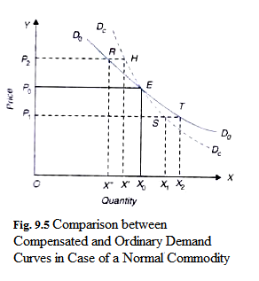
It will be seen from Fig. 9.5. that at a lower price P₁ together with compensation variation in income the consumer buys Ox₁ quantity of the commodity which corresponds to point S. Thus, point Sis the relevant point on the compensated demand curve corresponding to price P₁ and quantity Ox₁.

Now, suppose price of the commodity X rises from P₀ to P₂. In the absence of compensating variation in income, the consumer moves upward along the ordinary demand curve to point R and buys Ox” quantity and with this his real income will decrease as his new position will lie on a lower indifference curve than before. In order to keep his real income constant, if he is compensated by increase in money income, the quantity purchased of X by him will not decline as much as in the absence of compensating variation in income.

Therefore, with compensating variation in income his new equilibrium position will lie to the right of R, say at H, at which he buys Ox quantity of the commodity. By joining points such as H, E, S, we get a compensated demand curve along which real income remains constant. Thus, whereas along ordinary demand curve, a consumer’s money income remains constant, along compensated demand curve, his real income remains constant.

As is seen from Fig. 9.5 for a normal commodity, ordinary demand curve is flatter than compensated demand curve. This is because, as explained above, with the fall in price without compensating reduction in money income, the quantity purchased of a normal commodity will increase to a greater extent than what he buys when compensating reduction in income is made.

On the other hand, when price rises from P₀ to P₂, in the absence of compensating increase in his income, his quantity demanded of the commodity will decrease to a greater extent as compared to the quantity he buys when his money income is increased together with rise in price of the commodity so as to keep his real income constant.

However, it may be noted that the above condition that ordinary demand curve is flatter than the compensated demand curve is valid in case of normal goods. It may be recalled that normal goods are those whose demand increases when consumer’s income increases and vice-versa, that is, in their case income effect is positive. In case of inferior goods, the opposite is the case and for them ordinary demand curve is steeper than the compensated demand curve. This is because income effect in case of inferior goods is negative.

Measurement of Consumer Surplus with Ordinary and Compensated Demand Curves:

As noted above, the concept of compensated demand curve is needed to obtain the exact value of consumer surplus. Marshall measures consumer surplus as an area under the ordinary demand curve which includes the influence of both the substitution and income effects of price changes. The concept of consumer surplus is based on the marginal valuation of the units of a commodity and represents the excess of the sum of marginal valuations of the units of commodity purchased over the total price he pays for them.

Now, for the purpose of accurate measurement of marginal valuation of the commodity and therefore the consumer surplus which a consumer derives from his purchases, the concept of compensated demand curve is better than the ordinary demand curve as the former does not include the income effects of changes in price of a commodity. As explained above, the concept of compensated demand curve is based on the exclusion of income effect of price changes.

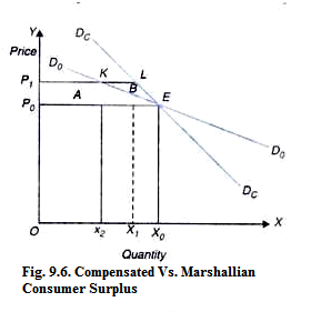
Let us illustrate with the help of a diagram how much error is introduced in the estimate of consumer surplus by using ordinary demand curve rather than compensated demand curve. In Fig. 9.6, we have reproduced the compensated demand curve D_CD_C ordinary demand curve D₀D₀ of a normal commodity. Suppose initially the price of commodity is P₀ at which the consumer is buying x_O quantity of the commodity on the ordinary the demand curve D₀D₀.

With the rise in price from P₀ to P₁ and the ordinary demand curve as the measure of marginal valuation, the consumer suffers a loss of welfare (as measured by decline in consumer surplus) by the area P₀ P₁ KE which is marked as A. However, if we use compensated demand curve, which more accurately represents marginal valuation of a commodity, loss of consumer surplus as a result of rise in price from P₀ to P₁ is equal to the area P₀P₁ LE (i.e., areas A + B) which is greater by the area marked as B than P₀P₁ KE obtained by using the concept of Marshallian ordinary demand curve concept.

It follows from above that in case of a normal commodity, the use of ordinary demand curve rather than compensated demand curve leads to the underestimation of the loss of consumer surplus. Likewise, in case of an inferior commodity use of ordinary demand curve rather than compensated demand curve leads to the overestimation of the loss of consumer surplus associated with a rise in price of a commodity.

It is worth mentioning that the difference in loss of welfare (i.e., consumer surplus) associated with the use of the concepts of compensated and the ordinary demand curves depends on the magnitude of income effect of the changes in price of the commodity. To the extent income effect is small,, the difference in welfare loss in using ordinary demand curve and compensated demand curve will tend to be small.

It should be noted that size of income effect of the changes in price depends on the importance of a commodity in consumer’s budget. Since in the actual world, for many commodities budget share spent on a single commodity is very small, income effect of price changes does not make much difference in the two cases. Therefore, in most cases, economists regard Marshallian measure of consumer surplus as a good approximation to the exact measure derived from the use of compensated demand curve.