Equilibrium in the Product Market and Money Market

Read this article to learn about the equilibrium in the product market and money market.

Equilibrium in the Product Market:

Equilibrium in the product market is reached when aggregate demand for output, i.e., C + i + G, becomes equal to aggregate supply of output (K) i.e., Y = C + ir + G.

At a given price level the consumers, businessmen and government are the demanders for output and the business sector is its supplier.

It is to be noted that every equilibrium level of output is related to a particular rate of interest. Because, change in interest rate brings about a change in the level of output or income through changing the level of investment.

Output to be in equilibrium, therefore, the rate of interest must also be in equilibrium at the same time. Rate of interest is an exogenous factor in the product market as it is determined in the money market. Product market therefore seeks to find the equilibrium values of the levels of output related to different interest rates.

One interest rate is related or associated with one equilibrium level of output and the other interest rate is related to another level of output. Thus, goods market equilibrium establishes various combinations of interest rate and output. A schedule of such combinations which show equilibrium points in the goods market is known as IS schedule.

The important condition for equilibrium in the goods market is that the total expenditure must be equal to output in the economy as shown in the equation given below.

Y = E = C + i + G …… (i)

or

Y = C[Y – T(Y)] + i + G …… (ii)

As the variables here are in real terms. Y = GNP, C is real consumer expenditure as a function of disposable income and T is real tax revenue as a function of real GNP, i is real intended investment and G is government purchases of goods and services. E stands for total expenditure.

Once GNP (Y) is produced generates equal amount of income (K) and is distributed amidst consumer expenditure, saving and taxes as shown by the following equation.

Y = C + S + T …… (iii)

or

Y – C = S[Y – T(Y)] + T (Y) ….. (iv)

where saving is a rising function of disposable income and tax revenue is a rising function of GNP (Y) On the basis of equation (i) and (iii) we can write:

C + i +G – C + S + T …… (v)

i + G = S + T …… (vi)

where i is the total investment showing intended investment plus change in inventories (∆inv). i + G is independent of income, whereas, S + T is a rising function of Y.

Equilibrium level of income will settle down only when S + T = i + G as shown by the following Fig. 12.1:

Producers keep a certain amount of output in stock for business purposes, known as inventories. Inventories are kept of a size considered ideal by the businessman or producers in the business sector. At Y₁, in Fig. 12.1 (S + T) > (i + G), showing excess supply over demand. Because of the fall in APC at higher levels of income, Y₁d is that part of output which was not purchased by the consumers. Out of Y₁d only a part i.e. Y₁c was purchased by the investors and government. Therefore, cd is unsold output which adds to the inventories which was not intended or desired by the businessman. There would be involuntary accumulation of inventories and the businessmen will cut down their orders for fresh production.

Through reverse action of multiplier income will be reduced to Y₀. When the economy is at Kn the APC is higher than it was at Y₁₁, resulting into low level of (S + T), where demand for output is greater than its supply. Excess demand will be met out of inventories. This will cause involuntary drop in inventories. In order to maintain a normal or an ideal level of inventories the sellers would issue fresh orders to the producers. This leads to the expansion of output or income up to Y₀ where (S + T) = (I + G), establishing equilibrium level of income. In the above analysis i, investment has been treated as fixed; whereas it does not remain fixed. It varies with the changes in interest rate. Investment, actually, depends upon two factors:

Firstly, it depends upon market rate of interest, because, it is a cost to the investors in either case whether the funds are borrowed or owned. Secondly, it depends upon the stream of future net returns from the project to be undertaken or the present discounted value (PDV) of the future net income from the investment to be made.

The PDV is computed by discounting the stream of future net returns at the market interest rate after deducting the cost (C) of the project, shown by the following equation:

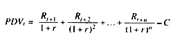
R_{t + 1} + R_{t + 2} etc. are net returns estimated at the time t i.e. t is time of taking decision regarding investment, r is the market rate of interest and C is the total cost of the project. If PDV is positive then it is beneficial to make investment otherwise not. In a project with positive PDV the investment will continue to flow in until it reaches zero. In the Fig. 12.2 projects have been arranged in order to their PDV counted on the basis of a fixed interest rate, say, r₀ or r₁.

When rate of interest is r₀ then investment will be made in six projects as all are having positive PDV_t raising the total investment up to i₀. When rate of interest falls to r₁ then the PDV_t curve shifts upward shown by dotted line in Fig. 12.2 This will make PDV_t of two more projects (7th and 8th) positive which will attract the investors, consequently, investment will rise up to i₁. Hence, there is functional relationship between interest, etc. and investment. Investment is an inverse function or r.

i = f(r) … (vii)

Thus investment is dependent on r, as r rises i falls and as r falls i rises.

Now, merging equation (vii) in equation (ii) we have

Y = C (Y – T (Y)) + i (r) + G …(viii)

Equation (viii) is a departure from Keynesian Model as it treats investment as variable and dependent on r. In the aggregate demand C and i depend on y and r respectively. At equilibrium level of output where AD = AS, there must be a pair of y and r. If either of the two undergoes a change the pair will be broken and a new equilibrium level of income will be achieved with a different pair of y and r. Equation (viii) therefore, establishes pairs of y and r that will maintain equilibrium in the product market.

 

Derivation of Is Curve:

By now we have come to know that there is opposite relationship between r and y. As r falls investment rises hence income (y) rises and vice versa. Fig. 12.3 shows the relationship between r and investment.

In Fig. 12.4 Equilibrium level of income is established by the intersection of (S + T) and (i (r₀) + G) functions at Y₀. As r₀ falls to r₁ the (i (r₁) + G) curve shifts upward due to rise in investment which intersects the (S + T) function at E₁ raising the equilibrium level of income to Y₁.

Thus, there is inverse relationship between y and r and the line or curve showing this relationship between the two must be negatively sloped. At a particular rate of interest there is a certain equilibrium level of y and that level of y will remain stable so long as that particular r does not change. This pair of r and y shows equili­brium in the product market. There can be several such pairs showing equilibrium in the product or goods market which can be shown by a curve known as IS curve. This can be shown by the Fig. 12.5.

In Fig. 12.5 r₀ is related with y₀ which shows equilibrium in the product market. As r falls to r₁ the equilibrium gets disturbed and new equilibrium is found at y₁, bringing (S + T) = [I(r₁) + G] and establishing equilibrium in the product market. IS curve comprises several such pairs of r and y.

All the relationships imbibed by IS curve and discussed so far can be shown together in a four quadrant (Fig. 12.6).There must be some equilibrium level of interest rate (r) in an economy at any point of time. From the equilibrium level of r we can trace the values of other variables in the diagram. Similarly, from other levels of r also we can find the values of these other variables.

In this four quadrant (Fig. 12.6) all the variables are rising from the origin and have positive values. Suppose r₀ is the equilibrium rate of interest and is given, measured on the vertical axis. At r₀ investment and government expenditure is (1 + G)₀ which through multiplier determines Y₀ equilibrium income. Y₀ is equilibrium income because here (S + T)₀ = (1 + G)₀. Note that (S + T) is a raising function of income, G is the amount of government expenditure which is fixed as it is independent of r.

At r₀ and y₀, (S + T)₁ = (1 + G)₀, the product market is in equilibrium as the equilibrium condition of income is satisfied here. The pair r₀ y₀ is shown by point A, a point on the IS curve. Similarly, at r₁ and Y₁ level of income (S + T)₁ =(1 + G)₁. Hence, r₁, v₁ is a combination which establishes equilibrium in the product market and shown by B. If we join AB points a curve comes into being known as IS curve, showing various combinations of r and y at which the product market is in equilibrium.

Shift In Is Curve:

An upward or downward shift in IS curve can take place if the factors like investment function, propensity to save, tax rate, interest rate etc. undergo a change. Effect of each can be seen separately. Shift due to increase in investment function: Suppose there is an upward shift in the investment function due to rise in the business expectations of the entrepreneurs. Its effect on the IS curve can be seen with the help of the Fig. 12.7.

IS is the original IS curve with pair r₀ y₀ where i’₀ = S₀ i. e- (i + G)₀ = (S + T)₀. The other pair is r₁ y₁ where i₁= s₁ (i + G)₁ = (S + T)₁ showing equilibrium in the product market. With an upward shift in the investment function to (i + G)₁ = ƒ(r) the level of investment goes up to i₁₁ i.e. (i + G)₁₁raising the level of income through multiplier to a level at which savings can be raised equal to i₁₁.

Income rises to y₁₁ at which i₁₁n or (i + G)₁₁ = (S + T)₁₁ at r₀ interest rate, making a new pair of r₀ y₁₁ which establish equilibrium in the product market. Another such pair results from the upward shift in the investment function is r₁ y₁₁₁ where i₁₁₁ = s₁₁₁ or (i + g)₁₁₁ = (S + T)₁₁₁. Thus, these new pairs i.e., r₀y₁₁ and r₁ y₁₁₁ in form a new IS curve resulting into upward shift in the IS curve. This implies that decline in the business expectations will shift the investment function downward and consequently the IS curve will also shift downward. Similarly increase and decrease in G will shift IS curve upward and downward respectively.

Shift due to Increase in Tax Rate:

Under the contractionary fiscal policy increase in tax rate (f) will shift the S + T function leftward or upward where every level of income will yield more S + T than before. For income to remain in equilibrium i + G must increase to match increased S+T.

This is possible only at lower rate of interest shifting the IS curve downwards as shown in Fig. 12.8. IS₀ is the original IS curve with combinations like r₀y₀ and r₁y₁ bringing equality between S+T and i + G and thus establishing equilibrium in the product market at various pairs of r and y lying on the IS0 curve. Increase in tax rate shifts the (S + T) function to (S + T)₁ shown by dotted line.

Now at y₀ more S + T takes place and therefore, for y to remain in equilibrium i + G must rise to match increased S + T which is possible only at r₁₁. New pair for equilibrium in product market is r₁₁ y₀ shown by A point. Similarly at y₁ the interest rate must fall to r₁₁₁ to bring equity between new S + T and i + G combination of y₁ r₁₁₁ is shown by B in Fig. 12.8. If we join A and B a new IS₁ curve is shaped by shifting the IS₀ downward. Decrease in tax rate, therefore, will shift the IS curve upward.

Effect of change in other variables like G, savings etc. can be worked out by the students themselves.

Equilibrium in the Money Market:

Schedule of the pairs of r and y fails to pin-point what exactly be the pair in an economy. This can be known if we know the equilibrium in the money market with r and y as its variable. For, any rate of interest on the IS curve may not be the equilibrium rate of interest. Equilibrium rate of interest is determined in the money market by the forces of demand for and supply of money.

The Demand for and Supply of Money:

Why do people have a demand for money? Simply because they need it for two kinds of purposes or requirements, known as transaction and speculative motives.

Transaction Motive:

People have to purchase articles of daily use like food, clothes, stationary etc. and make payments against them in money form. To do so they like to hold money balances with them. Holding of money for such purposes is known as transaction demand for money. Size of transaction demand for money depends upon two factors. First, more the time gap of one income receipt to another, larger the size of money holding would be required, on an average, to smooth out the time gap between income receipt and expenditure, and vice versa.

For instance, if Rs. 3,000 salary is paid per 10 days then average cash holding would be Rs. 1,500 only. This average money balance is between the time of the receipt of 3,000 at the beginning of 10 days and the time of zero money balance at the end of 10 days. Widening the time gap, if Rs. 9,000 is paid as monthly income then average cash demanded would be Rs. 4,500. It means wider the time gap between income receipts more is the demand for money.

Secondly, level of income also influences the transaction demand for money. Income and expenditure flows grow simultaneously is a fact. If monthly income grows to Rs. 18,000 the average demand for cash holding would rise to Rs. 9,000. However, the transaction demand for money depends upon the level of income.

M_t = K (Y); K > 0

K > 0 means there is positive relationship between money r demanded for transaction purposes (M,) and income level (V).

 

Money Demanded for Speculative Motive:

Another reason for which money is demanded is its capacity to invest. By investing in bonds people can earn interest or returns on bonds. Whenever interest on bonds rises they are lured to invest money in bonds and keep less cash balances with them. Because the opportunity cost of holding idle cash rises with the increase in interest rate. At very high interest rates money balances are squeezed to the minimum because, the opportunity cost of holding idle cash becomes very high. At very low interest rates their demand for such balances becomes infinitely high for the same reason. Such a demand for money, known as the speculative demand for money, depends upon the rate of interest.

M_s = L(r); L< 0.

L > 0 means there is opposite relationship between rate of interest and money demanded for speculative purposes (M_s).

Therefore, the total demand for money has two components and has been shown as demand for real money, computed by dividing the nominal money demand by the price level.

M^d/P= K(Y) + L(r)

It is only for analyzing the demand for money that it is divided into two kinds of demand for money. While deriving a total demand for money it is not wise to show the two kinds of demand separately. Because, one kind of demand affects the other. For instance, at high interest rates people may get lured to shift a part of their money holding from transactions to speculative re­quirements to earn interest and vice versa. So the total demand for money may be interpreted in the following equation.

M^d/P=ƒ(y,r)

Total demand for money (M^d) can be shown graphically. Total demand for money rises with the increase in income level as shown in Fig. 12.9. A given interest rate M^d rises and falls with the increase and decrease in income respectively as shown in Fig. 12.11.

As income rises from Y₀ to Y₁ the M^d curve shifts to M^d (Y¹) and the demand for money at r₀ rate of interest rises from M₀^d to M₁^d.

Supply of Money:

Supply of money is exogenously determined by the monetary authority and remains fixed over a period of time. It is not at all affected by the interest rate or it is interest insensitive as shown by the vertical line in Fig. 12.12.

 

Determination of Interest Rate:

Given the supply of real money (M^s/P ) equilibrium interest rate is determined where demand for money curve intersects the supply curve. There Fig. 12.12 shows r₀ as the equilibrium interest rate at Y₀ level of income. As income rises, market interest rate rises with the increase in income level i.e. from r₀ to r₁ as Y rises from Y₀ to Y₁. Reason for this is very simple. As Y rises people need more money for transaction purposes, therefore, they shift some money from speculative balances after withdrawing from interest earning bonds. This decline in the demand for bonds reduces the price of bonds and raises the interest rate. The suppliers of bonds would have to offer higher interest rates to find their buyers.

 

Derivation of the LM Curve:

After knowing the demand for and supply of money and the determination of interest rate in the money market, we can derive the LM curve. LM curve is a locus of all those combinations of Y and r where money demand is equal to the money supply. There can be several pairs of r and y where M^d, = M^s, showing equilibrium in the money market. If such pairs are joined we get a curve known as LM curve.

A four quadrant diagram has been used to derive the LM curve. Information relating to the transaction demand function K(Y) is provided by the lower left part, speculative demand function L(r) plus the transaction demand for money form the total demand for money (M^d = ƒ(Y, r) is shown by upper left part of Fig. 12.13. Vertical axis measures the interest rate, horizontal rightward axis and downward axis measure the levels of income. Horizontal leftward axis measures the demand and supply of money ,where M^d= M^s.

Suppose Y₀ is the equilibrium level of income. At Y₀ the transaction demand for money is M_t0 which is interest inelastic shown by its dotted line. After adding the speculative demand curve to this we get the total demand for money M^d at Y₀ shown in upper left part of the diagram. M^d at Y⁰ curve intersects the money supply line M^s ,which is interest inelastic, at r₀ rate of interest where M^d = M^s. This means that at r⁰ rate of interest and Y₀ level of income the money market is in equilibrium.

The pair of r₀Y₀ is shown by point A indicating a point on LM curve. Likewise, suppose income level is Y₁ creating M_t1 demand for transaction motive and to this is added the money demand for speculative motive shifting upward the total demand for money M^d at Y₁ shown in the diagram.

This M^d at Y₁ intersects the fixed money supply line at r₁ rate of interest where M^d = M^s. Thus r₁ and Y₁ is also a pair which establishes equilibrium in the money market and is shown by point B in the diagram as B. Joining of A and B forms a curve known as LM curve. Therefore, LM curve represents all those combinations of Y and r which maintain equilibrium in the money market. M^s and price level is fixed.

To take policy decision the question relating to the slope and position of LM curve is most important.

Slope of LM Curve:

Slope of LM curve means the responsive of interest rate (dr) to a given change in income (dy) (dr/dy). Change in the level of Y changes the demand for money for transacting motive. This changes money demand in speculative motive. How much interest rate changes to adjust this change in demand depends upon the elasticity of liquidity preference or of the money demand. Money demand can either be more or less sensitive or elastic to the changes in interest rate, depending on the psychology of the investors in bonds.

There can be three situations:

1. Interest elastic money demand,

2. Perfectly elastic money demand,

3. Perfectly interest inelastic money demand.

Interest Elastic Money Demand:

If the money demand is more elastic than the slope of the LM curve would be almost flat or less as shown in part A of Fig. 12.14. In another case if money demand is less interest elastic then the slope of LM curve would be steep as shown by part B.

Equal increase in Y in part A and B bring greater increase of r in part B and lesser in A. This is because in part A, M^d or money demand curve is more elastic resulting in almost Hat or less sloped LM curve. In part B money demand curve is less elastic. Increase in Y to Y₁ requires more money for transaction purpose which will flow out of speculative balances or bonds market.

This will reduce the demand for bonds in the bonds market, resulting in fall of the bonds prices and rise in interest rate. How much interest rate rises to spare the required money in transactions purposes? It depends on the elasticity of liquidity preference curve in speculative balances. In part B, it is clear that its elasticity is low, therefore, r has to rise much to absorb the changes in (M_t). Hence, LM curve would be steeply sloped. Contrary is in part A of Fig. 12.14.

 

Perfect Elastic Money Demand and Slope of LM Curve:

Keynes thought of an extreme case where the demand for money at minimum interest rate becomes perfectly elastic, popularly known as liquidity trap. In such a situation as the income level rises the demand for transaction purposes also rises but this increased demand for transaction purposes is met out of the idle money balances lying in the speculative motive.

Rate of interest does not increase at all to equilibrate the money market, because, the speculators at this minimum interest rate have already sold away their bonds expecting a fall in their prices in future. (Minimum interest rate means highest price of bonds). Hence, they hold cash money as much as possible. Interest rate remains stable even at higher levels of income as shown in the diagram below shaping a horizontal LM curve.

At Y₀ the total demand for money is M^d at Y⁰ shown in the left upper part of Fig. 12.15 which after intersecting the supply curve determines r₀ interest rate. The pair r₀Y₀ is shown by point A. As income, suppose, rises to Y₁, the M₁^d (money demand for transaction purposes) rises from M_t0 to m_t1 shifting the total demand for money to M^d at Y₁ which also intersects the money supply function at r₀. Rate of interest does not change at all to equilibrate the money market (M^d – M^r). Therefore, the new pair of r and Y becomes as r₀Y₁ shown by point B. Joining A and B gives a horizontal LM curve, also known as Keynesian Range.

Perfectly Inelastic Money Demand and Slope of LM Curve:

This is also an extreme case where demand for money is totally in responsive or inelastic to the changes in interest rate. It is a case where income has reached at full employment accompanied by a very high interest rate. At such a high r money demanded for speculative motive is zero as the investors believe that r will not rise any more (or prices of bonds will not decline). The entire money holding is used in transactions. It is a situation similar to classical economics. Level of r does not affect Y. The vertical LM curve is also known as Classical Range.

At Y₀ money demanded for transaction purposes (M_t^d) is equal to money supply M^s. It happens at very high interest rate such as r⁰ in Fig. 12.16, where money demanded for speculative motive is zero (M_s^d = 0) and the entire money (Ms) is used for transaction purposes (M_t^d) bringing money market in equilibrium (M_s = M_t^d), r is unaffected.

Slope of LM curve can be estimated by taking derivative of the equation for money market equations.

 

Shift in LM Curve:

LM curve can shift upward or downward if there are exogenous changes in the money supply (M^s) and money demand (M^d). Change in money demand can occur due to change in K i.e., the proportion of income kept as cash for transactions purposes. Change in M^d can also occur if there is increase or decrease in the speculative demand for money.

Some situations have been shown below:

Shift due to Increase in Money Supply:

LM function will shift downward and rightward as a result of increase in money supply. Because, the increased money supply will flow in the speculative motive which will reduce the rate of interest without any immediate change in income level. A pair with same income and lower r will result into shifting the LM curve as shown in Fig. 12.17.

LM is the original curve with r₀Y₀ and r₁Y₁ pairs with equilibrium in the money market. As money supply (M^s) is increased from M^s to M₁^s rate of interest falls to r₁₁ as M^d at Y⁰ interests the new supply curve (MI^s) at r¹¹. So a new pay of Y and r i.e., r₁₁Y₀ comes into being (A) while establishing equilibrium in the money market. Likewise such a new pair is formed with M^d at Y₁ level of income i.e., r₁₁₁Y₁ as shown by B. If we join AB we get a new LM₁ curve, if we decrease the money supply LM curve will shift leftward and upward. A shift in LM curve due to change in L (r) i.e., shift in LP curve and change in K (y) can be practiced by students themselves.