Elasticity of Supply: Meaning, Types, Measurement and Determinants

Let us make an in-depth study of the Elasticity of Supply. After reading this article you will learn about: 1. Meaning of Elasticity of Supply 2. Types of Elasticity of Supply 3. Measurement 4. Determinants.

Meaning of Elasticity of Supply:

The law of supply indicates the direction of change—if price goes up, supply will increase. But how much supply will rise in response to an increase in price cannot be known from the law of supply. To quantify such change we require the concept of elasticity of supply that measures the extent of quantities supplied in response to a change in price.

Elasticity of supply measures the degree of responsiveness of quantity supplied to a change in own price of the commodity. It is also defined as the percentage change in quantity supplied divided by percentage change in price.

It can be calculated by using the following formula:

E_S = % change in quantity supplied/% change in price

Symbolically,

E_S = ∆Q/Q ÷ ∆P/P = ∆Q/∆P × P/Q

Since price and quantity supplied, in usual cases, move in the same direction, the coefficient of E_S is positive.

Types of Elasticity of Supply:

For all the commodities, the value of E_s cannot be uniform. For some commodities, the value may be greater than or less than one.

Like elasticity of demand, there are five cases of E_S:

(a) Elastic Supply (E_S>1):

Supply is said to be elastic when a given percentage change in price leads to a larger change in quantity supplied. Under this situation, the numerical value of E_s will be greater than one but less than infinity. SS₁ curve of Fig. 4.17 exhibits elastic supply. Here quantity supplied changes by a larger magnitude than does price.

(b) Inelastic Supply (E_S< 1):

Supply is said to be inelastic when a given percentage change in price causes a smaller change in quantity supplied. Here the numerical value of elasticity of supply is greater than zero but less than one. Fig. 4.18 depicts inelastic supply curve where quantity supplied changes by a smaller percentage than does price.

(c) Unit Elasticity of Supply (E_S = 1):

If price and quantity supplied change by the same magnitude, then we have unit elasticity of supply. Any straight line supply Curve passing through the origin, such as the one shown in Fig. 4.19, has an elasticity of supply equal to 1. This can be verified in this way.

For any straight line positively-sloped supply curve drawn through the origin, the ratio of P/Q at any point on the supply curve is equal to the ratio ∆ P/∆ Q. Note that ∆ P/∆ Q is the slope of the supply curve while elasticity is (1/∆P/∆Q = ∆Q/∆P).Thus, in the formula (∆Q/∆P. P/Q), the two ratios cancel out each other.

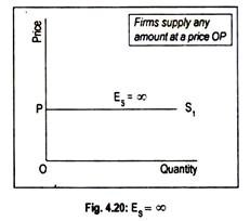
(d) Perfectly Elastic Supply (E_S = ∞):

The numerical value of elasticity of supply, in exceptional cases, may reach up to infinity. The supply curve PS₁ drawn in Fig. 4.20 has an elasticity of supply equal to infinity. Here the supply curve has been drawn parallel to the horizontal axis. The economic inter­pretation of this supply curve is that an unlimited quantity will be offered for sale at the price OS. If price slightly drops down below OS, nothing will be supplied.

(e) Perfectly Inelastic Supply (E_S = 0):

Another extreme is the completely or perfectly inelastic supply or zero elasticity. SS₁ curve drawn in Fig. 4.21 illustrates the case of zero elasticity. This curve describes that whatever the price of the commodity, it may even be zero, quantity supplied remains unchanged at OQ. This sort of supply curve is conceived when we consider the supply curve of land from the viewpoint of a country, or the world as a whole.

One important point to note here. Any straight line supply curve that intersects the vertical axis above the origin has an elasticity of supply greater than one (Fig. 4.17). Elasticity of supply will be less than one if the straight line supply curve cuts the horizontal axis on any point to the right of the origin, i.e. the quantity axis (Fig. 4.18).

Measurement of Elasticity of Supply:

Here we will measure the elasticity of supply at a particular point on a given supply curve. This is shown in Fig. 4.22 where SS’ is the supply curve.

To measure the elasticity of supply at a particular point on the curve SS’, we have drawn a straight line NT in such a way that it touches the SS’ curve at points A and C. As these two points lie very close to each other, the slope of the supply curve as well as the slope of the NT line is the same.

Following is the formula:

E_S = ∆Q/∆P.P/Q = AB/BC. OA/OQ

Triangles ABC and NQA are similar triangles.

Thus we can write NQ/QA instead of AB/BC.

Therefore,

E_S = NQ/QA. QA/OQ =NQ/OQ

As Fig. 4.22 suggests NQ < OQ, the coefficient of elasticity of supply is less than one i.e., inelastic.

If the NT straight line passes through the origin, the elasticity of supply becomes unity and if it passes through the price or vertical axis, the coefficient will be greater than one, i.e., elastic.

Determinants of Elasticity of Supply:

Here we are concerned with certain factors which affect elasticity of supply viz., the nature of the good, the definition of the good, the relevance of the time period, and so on.

(a) The Nature of the Good:

As with demand elasticity, the most important determinant of elasticity of supply is the availability of substitutes. In the context of supply, substitute goods are those to which factors of production can most easily be transferred. For example, a farmer can easily move from growing wheat to producing jute. Of course, mobility of factors is very important for such substitution.

As a general rule, the more easily the factors can be transferred from the production of one good to that of another, the greater will be the elasticity of supply. Since durable goods can be stored for a long time, its elasticity of supply is very high. But for non-durable goods and perishable goods elasticity of supply tends to be very low.

(b) The Definition of the Commodity:

As in the case of demand, elasticity of supply also depends on the definition of the commodity. The narrowly a commodity is defined the greater is its elasticity of supply. For example, it is easier for a tailor to transfer resources from producing red skirts to green skirts than from skirts to men’s trousers.

(c) Time:

Time also exerts considerable influence on the elasticity of supply. Supply is more elastic in the long run than in the short run. The reason is easy to find out. The longer the time period, the easier it is to shift resources among products, following a change in their relative prices.

This is usually true in the case of most agricultural commodities, because of the natural time lag between planting and harvesting of crops. In agriculture, production plans have to be made months or even years ahead and they cannot be altered quickly.

Manufacturing industries, on the other hand, can usually adjust their output upwards or downwards fairly quickly in response to changing conditions in the market.

Extractive industries come somewhere between the two:

Various types of mining, oil production and forestry can only alter their production plans slowly and, therefore, at any given time, have relative inelastic supply conditions.

Fig. 4.23 shows how time influences the supply of a commodity. If a very short period or momentary period is considered, the supply curve will be perfectly inelastic (Q₁S₁curve), where quantity supplied does not change even if price changes.

In the short run some degree of elasticity is found since supply can be adjusted to price change (SS₂ curve). SS₃ curve is a rather long run supply curve when quantity can be adjusted greatly to price change. As price increases from OP to OP₁ quantity supplied is unresponsive if the supply curve is Q₁S₁.

Quantity supplied increases to OQ₂ (> OQ₁) when the supply curve is SS₂ and quantity supplied rises to OQ₃ (> OQ₂ > OQ₁) if the supply curve is SS₃. Thus the supply of a commodity responds more, or is more elastic if a long time period is taken into account.

(d) The Cost of Attracting Resources:

If supply is to be increased it is necessary to attract resources from other industries. This usually involves raising the prices of these resources. As their prices rise, cost of production also increases. So supply becomes relatively inelastic.

If these resources can be obtained cheaply then supply is likely to be relatively elastic. These considerations become very important at times of full employment when the only available factors of production are those which can be attracted from other industries and uses.

(e) The Level of Price:

Elasticity of supply is also likely to vary at different prices. Thus, when the price of a commodity is relatively high, the producers are likely to be supplying near the limits of their capacity and would, therefore, be unable to make much response to a still higher price. When the price is relatively low, however, producers may well have surplus capacity which a higher price would induce them to use.