Economic Theories: 20 Economic Theories Formulated by Eminent Economists

Read this article to learn about the most popular economic theories formulated by eminent economist:

(1) J.B Clark’s Marginal Productivity Theory of Distribution, (2) Ricardo’s Theory of Rent, (3) J.B Clark’s Marginal Productivity Theory of Wage, (4) Classical Theory or Real Interest Rate Determination, (5) Neo-Classical Theory or Loanable Funds Theory, (6) Keynes’ Liquidity Preference Theory, (7) Francis L. Walker’s Rent Theory of Profit, and Others.

1. J.B Clark’s Marginal Productivity Theory of Distribution:

MP theory of distribution is used to determine the price of an input. For simplicity’s sake, we want to determine the price of labour i.e., wage rate. Anyway, this theory can be applied in the determination of any input.

The origin of the MP theory is rather obscure. However, J. B. Clark, an American economist, is greatly responsible for the popularisation of this theory in the late 1890s and early twentieth century. Jevons, Walras, Wicksteed, Marshall, Hicks, etc., have also given their own marginal productivity theories of distribution.

In certain respects, each version is somewhat different. Seeing different versions of the MP theory of distribution, Joseph Schumpeter, also an American economist remarked that there are as many marginal productivity theories as there are economists. Anyway, here we are concerned with the Clarkian presentation of the theory.

Clark’s Version:

J. B. Clark’s MP theory of distribution states that price of any input is determined according to the marginal product of that input. Thus, the price of labour—the wage rate—is determined by the volume of marginal product, or, to be more specific, the value of marginal physical product (VMP). Assuming a perfectly elastic supply of labour, wage of labour is determined in accordance with the VMP_L.

Since product market is characterised by perfect competition, VMP_L becomes equal to MRP_L. Thus, wage of labour tends to become equal to VMP_L =MRP_L. A competitive profit-maximising firm will go on employing labour until wage equals VMP_L = MRP_L i.e., W = VMP_L = MRP_L. This is the essence of the Clarkian version of the MP theory of distribution.

Assumptions:

Before presenting his theory, Clark made some simplifying assumptions abstracting from the real world. He assumed a completely static society where population, stock of capital, and techniques of production are constant.

Following are the important assump­tions of this theory:

i. Perfect competition exists both in product market and in input market. As a result, price of the product and price of the input are given.

ii. Every unit of input is homogeneous and easily substitutable.

iii. Inputs are perfectly mobile.

iv. There exists full employment of resources.

v. Employer can measure the marginal product of an input in advance.

vi. Law of variable proportions operates.

vii. Firm hires input with the objective of profit-maximisation.

viii. If all inputs are paid according to their marginal products total product would be exhausted—there would be neither surplus nor deficit.

Perfect competition in input market implies that neither input seller nor input buyer can influence the price of an input. At a given price, any amount of the input may be supplied. As a result, price of any input becomes equal to its average cost and marginal cost i.e., P = AC = MC. This means that the input supply curve must be perfectly elastic.

For the sake of analysis, we assume labour as the variable input. So, VMP_L=MRP_L curve is the labour demand curve. S_L = AC_L = MC₁ curve is the supply curve of labour.

Diagrammatic Representation of the Theory:

In Fig. 10.3 units of labour are measured on the horizontal axis and the price of labour i.e., wage rate or marginal product is measured on the vertical axis. Negative sloping labour demand curve (VMP_L=MRP_L = D_L) intersects the perfectly elastic labour supply curve (AC_L = MC_L = S_L) at point E. Point E is the equilibrium point because, at the going wage rate OW, the firm employs labour till wage rate equals VMP_L =MRP_L. In other words, the firm maximises profit by employing OL amount of labour at the wage rate OW. In fact, OW (=LE) is the marginal product of labour. Thus, wage of labour is determined by VMP_L= MRP_L.

OL is the profit-maximising level of employment because, at the ruling wage rate OW, the firm will not be able to maximise profit if it employs more than OL or it stops employment short of OL. If the firm hires less than OL units of labour at the wage rate OW, it means VMP_L = MRP_L > OW. So, it will be wise on the part of the firm to go on employing more labour until VMP_L=MRP_L = AC_L = MC_L.

Further, if the firm employs more than OL units of labour at the wage rate OW, VMP_L = MRP_L falls short of OW. This means that the marginal cost of labour is higher. So the firm will cut short of employment until VMP_L = MRP_L = AC_L = MC_L is reached. So, the profit-maximising firm should employ OL units of labour at the wage rate OW.

Labour, in this case, is the variable input while other cooperating inputs—say, land, capital and organisation, are the fixed inputs. Total output is, thus, the area under the VMP_L =MRP_L curve. Thus, the total production is the area OAFL. Out of this total output, the firm pays OWEL as wages and the rest (i.e., WAE) is being paid as the rewards of the other inputs in the form of rent, interest and profit. Thus, payment made in accordance with the marginal product exhausts the total product—there is neither surplus nor deficit.

However, this interpretation of the MP theory fails to determine the price of an input because input price is given or pre-determined. At a given wage rate OW, for an individual firm or industry, how many units of labour are employed can be known from this MP theory. In fact, what we have determined is the level of employment, given the wage rate. Thus, from the micro point of view, Clark’s theory is a theory of employment, rather than a theory of input price determination.

From a society’s point of view, what is pre­determined is the level of employment rather than the reward of an input. This is shown in Fig. 10.4 where we have drawn a perfectly inelastic supply curve of labour. This means that in the economy OL amount of labour is available. The supply of labour intersects the VMP_L = MRP_L = D_L curve at point E. Thus, E is the equilibrium point.

Equilibrium wage rate thus determined is OW —the marginal product of OL units of labour. Out of the total product OAEL, OWEL will be paid as wages and WAE will be paid as rent, interest and profit. Thus, total product gets exhausted. Given the labour supply, now we have determined the reward of labour i.e., wage. Thus, from the macro point of view, MP theory is a theory of input price determination.

Thus, the Clarkian presentation of the MP theory of distribution has two versions: from the micro point of view (i.e., from the viewpoint of a firm or an industry), Clark’s theory is an employment theory rather than a wage theory and from the macro point of view (i.e., from the viewpoint of an economy), this theory is a wage theory, rather than a theory of employment.

Criticisms:

Several criticisms have been leveled against this theory since most of the assumptions are unrealistic.

Following are the main criticisms against this theory:

In the first place, the MP theory of distribution becomes operative only when perfect competition exists. But, in reality, perfect competition does not exist either in the product market or in the input market. What we find in reality is the imperfect competition in both the product and input markets. This theory is inapplicable in the real world. In this sense, this is an unrealistic theory.

However, J. Robinson and E. Chamberlin have shown that Clark’s theory can be applied even in the imperfect market. In an imperfect market, inputs are rewarded less than their value of the marginal products. Thus, inputs are exploited. Inputs always get their ‘just’ shares provided perfect competition exists.

Secondly, inputs can never be homogeneous. Some inputs must be more efficient than others. Further, inputs are not easily substitutable. For instance, there are some inputs which are used in fixed proportions. In such a situation, no degree of substitution exists.

Thirdly, full employment of resources is another unrealistic assumption.

Fourthly, this theory assumes that the employer can measure the marginal product of an input in advance. Truly speaking, no employer measures marginal product either consciously or unconsciously. Further, if inputs are jointly demanded then calculation of marginal product of an input is virtually impossible.

Fifthly, this theory neglects the supply side of an input and describes only the demand side. Input is demanded because it is productive. But why is an input supplied cannot be answered from this theory since at a given price any amount of an input is supplied. Usually, an input is supplied more if it is remunerated more. This simple idea has not been considered by the authors of this theory. They merely describe why an input is demanded by a firm.

Sixthly, this theory cannot determine price of each and every input. Each input has certain peculiarities not found in others. Thus, the price of every input is not influenced solely by the marginal product. For instance, rent is greatly influenced by the inelasticity in the supply of land rather than its marginal product. Collective bargaining strength of a trade union has an important bearing on the wage rate. Profit is the result of risk and uncertainty borne by the entrepreneur rather than his marginal product.

Seventhly, total product gets exhausted if inputs are rewarded according to their marginal products. This is known as product exhaustion problem of the marginal productivity theory. Such product exhaustion takes place only when constant returns to scale operates. But constant returns to scale and perfect competition are incompatible. Further, under increasing returns to scale or diminishing returns to scale, total product does not get exhausted their occurs either deficit or surplus.

Finally, micro-presentation of the Clarkian version fails to determine the price of an input, since, from the micro point of view; it is an employment theory rather than a theory of input price determination. However, from the macro point of view, it is a theory of input price determination. Under this condition, the assumption of perfect competition in input market is absolutely redundant.

In view of these criticisms, this theory has been discredited. Today, there are few believers of this theory.

2. Ricardo’s Theory of Rent:

According to Ricardo, economic rent is enjoyed by land only. Rent arises due to the niggardliness of nature. According to Ricardo, rent is producer’s surplus. Rent is paid for the use of land whose supply is completely inelastic.

Ricordo’s theory is based on the following assumptions:

i. From the standpoint of the society, the supply of land is fixed. Thus, the supply of labour tends to become completely inelastic—its minimum supply price is zero in the sense that it supplies its working hours whether any payment is made or not.

ii. Law of diminishing marginal product operates.

iii. Malthus’ theory of population is operative. In brief, this theory states that a country’s population has the tendency to become double within 30 – 35 years.

iv. Land, being a gift of nature, has no cost of production. In view of this, rent does not enter into cost of production or price. Ricardo believed that price influences rent and not the other way.

Ricardo gave us a two-fold reason for the emergence of rent: (1) scarcity rent and (2) differential rent. Former type of rent arises due to the limited supply of land and the latter type of rent arises due to the differences in the productivity of land.

Scarcity Rent:

Let us assume that land available for cultivation is fixed and is therefore completely inelastic. Labour is the variable input. Let us also assume that marginal product of the variable input, labour, diminishes. As population tends to rise demand for land rises. So, according to Ricardo, rent must arise since supply of land is fixed in relation to demand. Consequently, prices of corn rise and surplus from land emerges. Such a surplus is Ricardo’s scarcity rent.

Land is fixed and homogeneous in quality. Land is used for the production of a single crop, corn. To explain Ricardo’s concept of scarcity rent, we use the following diagram. Panel (a) of Fig. 10.5 shows the equilibrium of an agricultural farm, while panel (b) shows the same for the market. SS is the market supply curve.

DD is the initial demand curve for the agricultural product that intersects the SS curve at point H. The market output, thus, determined is OQ and the corresponding price is OP. The corresponding equilibrium at the farm level occurs at point E where MC = MR = AC. A farm thus produces Oq and sells it at the price OP. Since P = AC, there is no surplus and, hence, no rent.

Let us assume that there is an increase in population following Malthusian logic. Thus, a rise in population results in an increase in the demand for corn. Market demand curve now shifts to D₁D₁ and it intersects the SS curve of point H₁. A higher price of corn (OP₁) thus results in and to feed more mouths now a pressure to increase production develops. Since land is fixed in supply, farms are now forced to increase production by making more intensive use of land.

At a higher price OP₁, the farm now produces Oq₁, where MC and AR₁ = MR₁ are equal. Since, revenues earned by the farm (OP₁Tq₁) exceeds cost (ONRq₁), the land, which was initially a free good, now has an economic value. Thus, the area NRTP₁ represents economic rent or surplus. Further, increase in the demand for corn following a rise in population will lead to an increase in the price of corn (OP₂—determined by the intersection of D₂D₂ and SS curves at point H₂) and, hence, increase in surplus or rent.

The volume of rent is, thus, determined by the price of the product. Thus, rent is a price- determined cost but not price-determining cost. This sort of rent has emerged due to the inelasticity in the supply of land.

Differential Rent:

It is quite likely that all lands are not of uniform quality. Truly speaking, lands are not homogeneous in quality; some lands are more fertile than others. Such differences in fertility or productivity of land result in the emergence of economic rent. This sort of economic rent has been described by Ricardo as differential rent.

For the sake of simplicity, we assume that in our society, there are three grades or categories of land where X is the superior and Z is the inferior land and Y grade of land lies between X and Z. In panel (d), market equilibrium has been shown. Product price is OP. The farm accepts this OP price. Ricardo assumed that a cultivator would produce first in the superior quality of land. As its supply is limited, the cultivator would then use next-best land whenever demand for corn rises consequent upon a rise in population.

Panel (a) of Fig. 10.6 shows that a farmer produces and sells Oq₁ output produced in superior-most land and enjoys a surplus or economic rent (the shaded area). As population rises, demand for corn rises. Since the supply of X-grade of land is fixed, people would then use Y- category of land—a less-superior land. Panel (b) shows that at a price OP the farmer sells Oq₂ output and enjoys a smaller volume of surplus (the shaded area).

Again, because of the population increase, farmer would now use inferior category of land where production becomes Oq₃. However, at the price OP, this output fails to yield any surplus and hence economic rent is zero (in panel c) since P=AC. Ricardo called this inferior or category-Z land as the marginal land. Marginal land does not yield any rent. Rent, thus, arises only in superior land (here X- category) and intra- marginal land (here Y- category) — land that lies between superior and marginal land.

Now, if demand for corn rises, price will rise. Consequently, rent will rise. Note that, as demand curve shifts to D₁D₁, price of corn rises to OP₁. Consequently, surplus or economic rent increases in all grades of land. Now the marginal land or no-rent land yields economic rent and this land becomes intra-marginal land. Thus, rent is a price- determined cost, but not a price-determining cost. As price of corn rises, rent rises.

Further, economic rent is an ‘unearned surplus’ since rent is governed by the price of corn.

Limitations:

Ricardo’s theory of rent is subject to criticisms.

They are:

i. First, it may be objected that land does not have any original and indestructible powers. Such power of land can be changed through scientific way.

ii. It is unrealistic to assume that land has only one use. Instead, land has alternative uses. It can be used for variety of purposes. As Ricardo assumed that land has only one use its supply is completely inelastic. A particular plot of land may be used for the production of either wheat or jute. As land has alternative uses, the supply of land to a particular use cannot be addressed as perfectly inelastic.

iii. Lands are never cultivated in descending order of fertility as was assumed by Ricardo. Actually, cultivation is pursued in accordance with the location of land and other reasons.

iv. The concept of marginal or no-rent land is not found in reality.

v. According to Ricardo, rent is specific to land. In other words, rent arises only in the case of land. But modern economists have demonstrated that rent arises not only in the case of land but also in the case of other factors of production.

vi. Finally, Ricardo has shown that rent is determined by the rice of corn. That is to say, in Ricardo’s theory rent does enter into cost of production. This Ricardian idea becomes true if we consider the supply of land from the viewpoint of the economy as a whole. If supply of land is considered from the viewpoint of a firm or industry, rent then determines price and, hence, rent will enter cost of production.

Modern Theory of Rent:

Modern economists have generalised the concept of rent, though it was Ricardo who first propounded the theory of rent and applied it to land only. Modern economists argue that supply of all inputs is more or less inelastic. So, rent is enjoyed by all inputs including land.

An alternative definition of rent has been given by modern economists. Economic rent is defined as the difference between actual earnings and transfer earnings or minimum supply price of any input. Actual earnings are the earnings what an input actually earns after rendering services for a given period of time. Transfer earnings are the payment that must have to be paid to keep an input in its present use.

Transfer earning or the minimum supply price is the price that must have to be paid to an input in order to retain its job. Thus, economic rent is a payment to any input over and above what is required to keep the input in its current employment. In other words, economic rent is any payment in excess of transfer earnings or minimum supply price or opportunity cost.

Transfer earnings are regarded as opportunity cost of keeping a factor of production in its present use or it is regarded as the input’s supply price in its present occupation. Whenever an input does not have an alternative use, its opportunity cost becomes zero. Thus, the entire earnings of that input become rent.

The volume of economic rent depends on the elasticity of supply of any input. Let us assume that the supply of labour is perfectly inelastic as drawn in Fig. 10.7. In the short run, the supply of labour may be completely inelastic. Here SS₁ is the supply curve whose coefficient of elasticity of supply is zero. This means that whatever the price, its supply is always OS. Even if the input is not rewarded its supply would be fixed at OS.

That is why, the supply curve of this input is completely inelastic (e_s = 0). Actual earnings (AE) of an input are determined by the intersection of the demand curve for an input and the supply curve of that input. Thus, the actual earning of the input becomes equal to OPES. Since opportunity cost or minimum supply price (MSP) is zero, the entire earnings of the input are economic rent (i.e., OPES).

In Fig. 10.8, we have drawn a perfectly elastic supply curve of labour, PS. This means that at a given price OP, any amount of labour will be supplied. Thus, the minimum supply price of that input is OP. Actual earnings are determined by the intersection of DD curve and PS curve at point E. Actual earnings now equal to OPEA. Since actual earnings and opportunity cost are the same, labour does not enjoy any amount of economic rent.

In case of an upward rising supply curve of an input, part of its earnings become rent. In Fig. 10.9, we have drawn a positively sloped supply curve of labour, SS₁. Its slope indicates that as price of labour increases, its supply increases. Demand curve DD intersects the supply curve SS₁ at point E. Actual earnings are, therefore, OPEM. Now these actual earnings can be split into two parts: opportunity cost and the economic rent. Suppose, OM₁-th unit of labour is supplied whose opportunity cost is the area under the supply curve, i.e., M₁N₁.

Its actual earnings are M₁P₁ (= OP). Thus, the OM₁-th unit of labour earns rent to the tune of P₁N₁ or SN₁P₁P area. Similarly, OM₂-th unit of labour enjoys rent of P₂N₂ amount since actual earnings (M₂P₂) exceed opportunity cost (M₂N₂). For the OM-th unit of labour since actual earnings and opportunity cost are equal, no economic rent accrues. In other words, OM-th unit of labour does not receive any surplus or economic rent. But, for OM units of labour, opportunity cost or minimum supply price equals OSEM area, while actual earnings are OPEM. Thus, OM units of labour get rent to the extent of PSE.

Thus, we can conclude that the volume of economic rent depends on the elasticity of supply of any input. Greater the elasticity of supply, lower is the economic rent, and lower the elasticity of supply, greater is the economic rent.

Finally, modern economists challenged Ricardion contention—rent is price-determined but not price-determining. This Ricardo’s view is correct only when the supply of land is viewed from the society’s angle. In this situation, opportunity cost is zero, since land has no alternative use. In such a situation, rent is price- determined. But, from a firm’s or industry’s point of view, opportunity cost is positive. So, rent will then determine price and not the other way, as Ricardo argued.

3. J.B Clark’s Marginal Productivity Theory of Wage:

The marginal productivity theory of wage states that price of labour i.e., wage rate is determined according to the marginal product of labour. This was stated by neo-classical economist, especially J. B. Clark, in the late 1890s. The term marginal product of labour is interpreted here in three ways: marginal physical product of labour (symbolised by MPP_L), value of the marginal product of labour (symbolised by VMP_L) and marginal revenue product of labour (symbolised by MRP_L).

When marginal product of labour is expressed in money terms we obtain VMP_L. MRP_L is the change in total revenue following a change in the employment of labour. Marginal productivity theory of wage states that wage of labour equals VMP_L (= MRP_L). Employer will employ labour up to the point until market wage equals labour’s value of the marginal product and marginal revenue product.

Assumptions:

Following are the important assumptions of this theory:

i. Perfect competition prevails in goods market and in labour market. Perfect competition in goods market implies that goods produced are homogeneous and the price of the goods is given for all firms in the market. Perfect competition in labour market also implies that labour as well as firms behave as ‘wage-taker’s. No one can influence the wage rate. Consequently, labour supply curve, S_L, becomes perfectly elastic. Since wage rate does not change, labour supply curve incidentally becomes the average cost curve of labour (AC_L), and it coincides with the marginal cost curve of labour (MC_L).

ii. Law of variable proportions operates.

iii. The firm aims at profit maximisation.

iv. All labourers are homogeneous and are divisible.

v. Labour is mobile and is substitutable to capital.

vi. Resources are fully employed.

Wage rate will be determined by the interaction of demand and supply curves of labour in the market. Labour demand curve is explained by the VMP_L curve. Since perfect competition exists in the product market, VMP_L curve coincides with the MRP_L curve. VMP_L = MRP_L curve is the firm’s demand curve for labour. This curve slopes downwards because of diminishing marginal returns. In Fig. 10.11, VMP_L = MRP_L = D_L represents a firm’s demand curve for labour.

Further, as perfect competition exists in the labour market, the labour supply, S_L = AC_L = MC_L, curve has been drawn perfectly elastic.

In Fig. 10.11, E is the equilibrium point since, at this point, labour demand equals labour supply. The equilibrium wage rate thus determined is OW. Corresponding to this wage rate, equilibrium level of employment is OL. Note that, for OL amount of labour, VMP_L = MRP_L is LE, which equals wage rate OW. At this going wage rate (i.e., OW) the employer will be maximising profit by employing OL units of labour. However, less (more) labour will be employed if market wage rate rises above (falls below) OW.

Limitations:

This neo-classical theory of wage is subject to a large number of criticisms. Most of the criticisms of this theory are directed against the assumptions. Most of the assumptions are unrealistic.

The main criticisms are explained below:

i. In the real world, perfect competition does not exist both in product market and in labour market. Imperfect competition is found in all the markets. This theory, therefore, has the limited applicability in the real world. If it is applied to the imperfectly competitive market, worker will be subject to exploitation.

ii. Labour can never be homogeneous— some may be skilled and some may be unskilled. Wage rate of a worker is greatly influenced by the quality of labour. A higher wage rate is enjoyed by the skilled labour compared to the unskilled labour. This simple logic has been totally ignored by the authors of this theory.

iii. Perfect mobility of labour is another unrealistic assumption. Mobility of labour may be restricted due to socio­political reasons.

iv. The marginal productivity theory of wage ignores supply side of labour and concentrates only on the demand for labour. It is said that labour is demanded because labour is productive. But why labour is supplied cannot be answered in terms of this theory. This is because of the fact that, at a given wage rate, any amount of labour is supplied. But, we know that higher the wage rate higher is the supply of labour. This positive wage- labour supply relationship has been ignored by the makers of this theory.

v. Full employment of resources is another unrealistic assumption.

vi. This theory, in fact, is not a wage theory but a theory of employment. Wage rate is pre-determined. At the given wage rate OW, how many units of labour are supplied can be known from this theory.

v. In this sense, it is a theory of employment and not a theory of wages.

vi. Finally, this theory ignores the usefulness of trade union in wage determination. Trade union, through its collective bargaining power, also influences wage rate in favour of the members of the organisation.

In view of all these criticisms, the marginal productivity theory of wages has become useless.

4. Classical Theory or Real Interest Rate Determination:

Regarding the nature of interest, classicists were not unanimous. They regarded the nature and the determinants of the rate of interest in terms of a more complex pattern. Some classical economists like A. Marshall, N. W. Senior, Bohm-Bawerk, I. Fisher, etc., viewed interest from the supply side of capital i.e., saving. On the other hand, economists like J. B. Clark explained the nature of interest from the viewpoint of the demand for capital i.e., investment. Since demand for and supply of capital are composed of real factors, classical theory is regarded as the real interest rate theory.

i. Supply of Capital or Saving:

According to N. W. Senior, saving involves a sacrifice. People abstain from consumption. Since abstinence involves a sacrifice, savers must be rewarded in the form of interest. This is called abstinence theory of interest. Because of criticism made by Karl Marx against the concept of abstinence, Marshall substituted the term ‘waiting’ for abstinence.

Marshall’s theory is regarded as the waiting theory or interest. According to this theory, whenever money is lent by an individual he has to wait to get back his money. As he ‘waits’ for future he has to be given interest. Thus, interest is the price for waiting. Higher the interest, higher is the period of waiting. In other words, people will save more if they are rewarded more. Thus, supply of capital comes from saving.

Bohm-Bawerk, Fisher, etc., provided another theory that also governs the supply of capital. Their theories are popularly known as ‘time preference theory of interest.’ According to them, as people prefer current consumption over future consumption, they become impatient to spend money now. To make future consumption more profitable, an individual must be given inducement in the form of interest income.

Thus, supply of capital is dependent on real or psychological factors like (i) abstinence, (ii) waiting, and (iii) time preference. Obviously, higher the rate of interest greater is the volume of savings. In other words, saving or supply of capital is directly related to the rate of interest. Thus, the saving function becomes

S = f(r)

ii. Demand for Capital or Investment:

The principle of marginal productivity can be employed in determining the volume of investment. Like other inputs, capital has marginal productivity. According to the marginal productivity theory of capital, which is a part of marginal productivity theory of distribution, price of capital is determined in accordance with the marginal revenue product. Marginal revenue product of capital or demand for capital or investment will rise if the rate of interest declines. Investment demand is inversely related to the rate of interest. Thus, investment function becomes

I = f(r)

Since supply of capital or saving function is positively related to the interest, the saving curve SS has been drawn upward sloping in Fig. 10.12. Investment curve II has been drawn downward sloping. Equilibrium rate of interest is determined at point E the point at which investment and saving curve intersect each other. Or is the equilibrium rate of interest which brings savings (OK) into balance with investment (OK).

Criticisms:

Classical theory of interest rate determination has come in for sharp criticisms:

i. This theory is based on full employment assumption. But, what we find in reality is the unemployment or under­employment of resources. Classical theory does not work below full employment.

ii. Keynes charged the classical theory as an indeterminate one. According to Keynes, saving depends on income level. There will be different saving schedules at different income levels. As income rises saving curve shifts upward. Thus, we cannot know the position of the saving curve unless we know the level of income and, if we do not know the volume of savings, we cannot determine interest rate.

Thus, interest rate remains indeterminate if the level of income is not known. But we do not know the level of income without knowing the interest rate because it is the rate of interest that brings about a change in investment and income level. Hence the indeterminacy in the interest rate.

iii. Finally, according to Keynes, rate of interest is determined by the monetary factors rather than by real factors.

5. Neo-Classical Theory or Loanable Funds Theory:

An improved version of classical interest rate theory was provided by neo-classical economists like K. Wicksell, D. H. Robertson. This theory has come to be known as the loanable funds theory. This theory holds that the rate of interest, like any other price is determined by the demand for and the supply of loanable funds. This theory further holds that the rate of interest is not determined alone either by real factors as assumed by the classicists or by monetary factors as assumed by Keynes. In fact, both real and monetary factors determine interest rate.

Sources of Supply of and Demand for Loanable Funds:

Now we consider sources of supply of and demand for loanable funds.

(a) Supply of Loanable Funds:

By loanable funds we mean money available for lending in financial markets.

There are three sources of supply of loanable funds:

(a) Savings

(b) Dishoarding of money from past savings, and

(c) Bank created money.

i. Savings:

Households and firms supply loanable funds in the capital market out of their savings. Savings are the surplus over consumption. This theory assumes that given the level of income, savings vary directly with the rate of interest. In Fig. 10.13, savings have been represented by the ‘S’ curve which is interest-elastic.

ii. Dishoarding from past savings:

Individuals hoard cash from their previous incomes. If now these hoarded wealth are dishoarded, idle money (i.e. hoarded money) now becomes active money and, therefore, supply of loanable funds rises. If more interest is given people will be induced to dishoard their wealth in order to earn more interest income. The curve ‘DH’ represents this element of loanable funds.

iii. Bank money:

Commercial banks provide money in the economy. Banks advance loans to the public by creating credit. Obviously, more money will be injected into the economy if banks earn more interest income. At a low rate of interest, the willingness to lend money by the banking system declines. The supply curve of money has been represented by ‘∆M’ curve.

By lateral summation of all these sources of loanable funds, we obtain total supply of loanable funds in the financial markets:

S_Lf = S + DH + ΔM

where S_Lf represents supply of loanable funds. The curve S_Lf is the supply curve of loanable funds. This curve has an upward slope indicating that its volume rises as interest rate rises.

(b) Demand for Loanable Funds:

Like supply of loanable funds, demand for loanable funds arises from three sources. They are: (a) investment, (b) dis-saving, and (c) hoarding.

i. Investment:

In the loanable funds theory, investment demand is governed by the marginal revenue productivity of capital. Since the productivity curve has a negative slope, investment demand is inversely related to the rate of interest. The ‘I’ curve represents this element of demand for money.

ii. Dis-saving:

Demand for loanable funds arises from consumption. People take loans to finance their consumption activities. Dis-saving or consumption is inversely related to the rate of interest. ‘DS’ curve represents this element of demand for loanable funds.

iii. Hoarding:

Hoarding is another source of demand for loanable funds. Demand for hoarding money arises from preference for liquidity or in short, liquidity preference. As liquid cash is attractive, people hoard money. Demand for hoarding money also depends on the interest rate. At a higher rate of interest, willingness to hoard money on the part of individuals, business firms, etc. declines while willingness to lend money rises. Such relationship between hoarding of money and interest is depicted by the curve ‘H’ in the Fig. 10.13.

By summing up all these sources of demand for loanable funds we obtain total demand for loanable funds. Thus,

D_Lf= I + DS + H

where D_Lf represents total demand for loanable funds. The curve D_Lf represents this.

In Fig. 10.13, DH, ∆M and S curves are upward sloping curves showing a positive relationship between them and interest rare. When all these elements are added together we get positive sloping S_Lf curve. Similarly, negative sloping D_Lf curve has been drawn on the basis of summation of DS, H and I curves. These two curves intersect each other at point E and the equilibrium rate of interest, thus, determined is ‘Or’. The interest rate brings demand for and supply of loanable funds in balance.

Limitations:

One of the chief merits of this neo-classical loanable funds theory is that it is an improvement over the classical theory of interest rate determination. Unlike the classical theory, it does not include only savings as the source of loanable funds. Further, it considers monetary factors like bank money and dishoarding as the two major sources of loanable supply of funds.

Keynesian interest rate theory is purely a monetary theory. Neo-classical loanable funds theory again scores marks over the Keynesian theory as this theory emphasises on real factors, such as savings, marginal productivity of capital or investment to determine interest rate. But this does not mean that this theory is fault-free. It has too certain strongest limitations.

These are the following:

i. Like the classical theory, this theory assumes a fixed money income. Given income, a change in interest rate brings about a change in the savings and investment. As interest rate rises, saving rises. But, Keynes argued that an increase in interest rate means a fall in investment. Fall in investment leads to a fall in income and hence ultimately fall in savings.

ii. Keynes charged this theory on the ground that, like the classical theory, it cannot provide a determinate solution to the interest rate determination. Without knowing the income level the supply of loanable funds remains unknown, and without knowing the supply of loanable funds rate of interest remains indeter­minate. In other words, we cannot determine the rate of interest unless we know the level of income. Hence indeterminacy.

iii. The theory is based on unrealistic assumption of full employment of resources.

iv. Saving in modern days is often influenced by habit and custom as well as security, irrespective of the rate of interest.

However, this theory assumes a direct relationship between saving and interest.

In view of these reasons, the loanable funds theory has little to say in policy formulation.

6. Keynes’ Liquidity Preference Theory:

The determinants of the equilibrium interest rate in the classical model are the “real” factors or the supply of saving and the demand for investment. On the other hand, in the Keynesian analysis, determinants of the interest rate are the “monetary” factors. Keynes’ analysis concentrates on the demand for, and supply of, money as the determinants of interest rate. According to Keynes, the rate of interest is purely “a monetary phenomenon.” Interest is the price paid for borrowed funds.

People like to keep cash with them rather than investing cash in assets. Thus, there is a preference for liquid cash. People, out of their income, intend to save a part. How much of their resources will be held in the form of cash and how much will be spent depend upon what Keynes calls ‘liquidity preference’. Cash being the most liquid asset, people prefer cash. And interest is the reward for parting with liquidity. However, the rate of interest in the Keynesian theory is determined by the demand for money and supply of money.

Factors Determining Rate of Interest:

i. Demand for Money:

By demand for money, we mean demand to hold an asset.

The desire for liquidity or demand for money arises because of three motives:

(a) transaction motive,

(b) precautionary motive, and

(c) speculative motive.

ii. Transaction demand for money:

Money is needed for day-to-day transactions. As there is a gap between the receipt of income and spending money is demanded. Since payments or spending are made throughout a period and receipts or incomes are received after a period of time, an individual needs ‘active balance’ in the form of cost to finance his/her transactions. This is known as transaction demand for money which directly depends on the level of income of an individual and businesses.

Symbolically,

T_dm = f(Y)

where T_dm stands for transaction demand for money and Y stands for income.

iii. Precautionary demand for money:

Future is uncertain. That is why people hold cash balances to meet unforeseen contingencies, like death, accidents, danger of unemployment etc., The amount of money held under this motive called ‘idle balances’—also depends on the level of income of an individual. The relationship between precautionary demand for money (P_dm) and the volume of income is normally direct. Thus,

Pdm = f(Y)

iv. Speculative demand for money:

This sort of demand for money is really Keynes’ contribution. The speculative motive refers to the desire to hold one’s assets in liquid form to take advantages of market movements regarding the uncertainty and expectation of future changes in the rate of interest. The cash held under this motive is used to make speculative gains by dealing in bonds and securities whose prices and rate of interest fluctuate inversely.

If bond prices are expected to rise (or the rate of interest is expected to fall) people will now buy bonds and sell when their prices rise to have a capital gain. In such a situation, bond is more attractive than cash. Contrarily, if bond prices are expected to fall (or the rate of interest is expected to rise) in future people will now sell bonds to avoid capital loss.

In such a situation, cash is more attractive than bond. Thus, at a low rate of interest liquidity preference is high and at a high rate of interest securities are attractive. Now, it is clear that the speculative demand for money (S_dm) varies inversely with the rate of interest. Thus,

S_dm = f(r)

where ‘r’ is the rate of interest.

v. Total demand for money:

The total demand for money (DJ is the sum of all three types of demand for money. That is, D_M = T_dm + P_dm + S_dm. The demand for money has a negative slope because of the inverse relationship between the speculative demand for money and the rate of interest. However, the negative sloping liquidity preference curve becomes perfectly elastic at a low rate of interest.

According to Keynes, there is a floor interest rate below which rate of interest cannot fall. This minimum rate of interest indicates absolute liquidity preference of the people. This is what Keynes called ‘liquidity trap’. In Fig. 10.14, D_m is the liquidity preference curve. At minimum rate of interest, r-min, the curve is perfectly elastic. However, there is a ceiling of interest rate, say r-max, above which it cannot rise. Thus, interest rate fluctuates between r-max and r-min.

vi. Money Supply:

The supply of money in a particular period depends upon the policy of the central bank of a country. Money supply curve, S_M, has been drawn perfectly inelastic.

vii. Determination of the Rate of Interest:

According to Keynes, rate of interest is determined by the demand for money and supply of money. OS is the total amount of money supplied by the central bank. At point E, demand for money becomes equal to the supply of money. Thus, the equilibrium interest rate is determined at ‘Or’. Now, suppose rate of interest is greater than ‘Or’. In such a situation supply of money will exceed the demand for money. People will purchase more securities. Consequently, its price will rise and interest rate will fall until demand for money becomes equal to the supply of money.

On the other hand, if the rate of interest becomes less than ‘Or’, demand for money will exceed the supply of money, people will sell their securities. Price of securities will tumble and the rate of interest will rise until we reach point E.

Thus, the rate of interest is determined by the monetary variables only.

Limitations:

Keynes’ liquidity preference theory is also not free from criticisms.

First like the classical and neo-classical theories, Keynes’ theory is an indeterminate one. Keynes charged the classical theory on the ground that it assumed the level of employment fixed. Same criticism applies to Keynes since he assumes a given level of income. Keynes’ theory suggests that D_m and S determine the rate of interest. Without knowing the level of income we cannot know the transaction demand for money as well as speculative demand for money.

Obviously, as income changes, liquidity preference schedule changes, leading to a change in the interest rate. Therefore, one cannot determine the rate of interest until the level of income is known, and the level of income cannot be determined until the rate of interest is known. Hence indeterminacy. Hicks and Hansen solved this problem in their IS-LM analysis by determining simultaneously the rate of interest and the level of income.

Secondly, Keynes committed an error in rejecting real factors as the determinants of interest rate determination.

Thirdly, Keynes’ theory gives a choice between holding risky bonds and riskless cash. An individual holds either bond or cash, and never both. In the real world, it is the uncertainty or risk that induces an individual to hold both. This gap in Keynes’ theory has been filled up by James Tobin. In fact, today people make a choice between a variety of assets.

7. Francis L. Walker’s Rent Theory of Profit:

Rent theory of profit—as developed by Francis L. Walker—says that pure or net profit is the rent of ability. Just as land is heterogeneous in quality, entrepreneurs are also of different qualities. Rent arises due to differences in productivity of lands. Rent arises in the case of superior or intra-superior land. Rent does not arise in the case of marginal land.

According to Walker, this is also true of entrepreneurs. Some entrepreneurs, say superior ones, earn profit while inferior or marginal entrepreneurs do not earn any profit. Thus, profit is attributed to the differences in ability. Like rent, profit is a differential surplus which accrues to the superior or intra-superior entrepreneurs.

Criticisms:

i. Profit may arise due to differences in ability. But profit may arise due to monopoly, innovation, risk, etc. Walker ignores all these elements.

ii. Walker’s logic is not convincing when he says that the marginal entrepreneurs are non-profit earners and therefore profit does not enter into price. In economics, normal profit is included in the cost of production and therefore enters into price.

iii. The concept of no-profit entrepreneurs as envisaged by Walker is rather an unrealistic one. Profit is the best guide for an entrepreneur to stay in business. If marginal entrepreneurs do not get profit, what is their incentive to stay in business. They should shut down their businesses. This does not happen in real world.

iv. In modern business, there has been a separation of ownership from management. Owners or the share­holders earn dividends—whether they are superior or not. So, profit is not the result of rent of ability even if the sleeping shareholders get profit in the form of dividends.

v. Finally, profit is the result of managerial function. An organiser is supposed to manage, coordinate various functions. But, at the same time, the organiser undertakes risk. Profit arises because organiser undertakes risk. This important function has been ignored by Walker.

In view of all these criticisms, there is not a single believer of this theory.

8. Davenport and Taussig’s Wages Fund Theory:

Davenport and Taussig’s name are associated with the wage funds theory. According to Taussig, profits are regarded as simply a form of wages. They accrue to the entrepreneur on account of his special ability. Therefore, profit is not a chance income; it arises due to special skill possessed by the entrepreneur. As skill is the characteristic of labour, profits of the entrepreneurs should be regarded as wages. Since an entrepreneur is a special class of factor of production, he must receive profit.

Criticisms:

i. This theory finds an equivalence between wages and profit. But, we know that wages are earned income—the result of toil and work; while profit is the result of a variety of things, including a ‘chance’.

ii. Workers get wages so long as they work. But profit is an uncertain income. It may be zero or even negative.

iii. Shareholders, without performing any economic function, earn profit. This theory cannot explain this phenomenon.

iv. Profit may arise due to (i) imperfection, (ii) innovation, (iii) risk taking, etc. Walker did not appreciate these elements.

In view of these criticisms, one can label this theory as a highly unsatisfactory theory.

9. J.B. Clark’s Dynamic Theory of Profit:

J. B. Clark propounded that profit arises in a dynamic society. In other words, profit does not arise in a static economy. A stationary economy is characterised by unchanged size of population, supply of capital, the methods of production, the organisation of business, etc. Thus, a static economy is a changeless economy. According to Clark, five generic changes go on, everyone of which reacts on the structure of society.

In a dynamic state, population increases, capital increases, methods of production change or improve, forms of business organisation change, quantity and quality of human wants change. We know that profit is a surplus beyond full cost of production. It is defined as the difference between selling price and, hence, total revenue and total cost. In a changeless economy, there does not occur any difference between revenue and cost; price tends to equal cost. Consequently, profit disappears. Profit is, thus, the result of five dynamic changes.

Criticisms:

i. There is no guarantee that a dynamic society always earns profit. We live in a changing world where variety of changes take place. Under the circumstances, one finds lot of loosing firms. So, profits are not to be attributed to changes alone.

ii. Clark emphasises too much on changes and neglects managerial function of an entrepreneur. An efficient manager may earn profit if he performs his functions efficiently. So, profit is the result of entrepreneurial function.

iii. No economy is a static one. An efficient innovative entrepreneur always brings about a change. Obviously, profit will arise. It is to be remembered that all changes may not give rise to profit. Only those changes which are unpredictable may give rise to profit.

iv. Profit may arise due to risk-taking. Clark did not find any relation between risk- taking and profit.

10. Hawley’s Risk and Uncertainty Theory of Profit:

People go into business with the hope of getting profit. But the future is uncertain. In this uncertain world, nothing works out in accordance with the plans and targets the business makes. Business decisions are made and actions are taken. Because of uncertainty, such actions may be right and so profits may arise. If such actions prove to be wrong, losses arise. Thus, profit is the consequence of uncertainty.

According to F. B. Hawley, the main function of an entrepreneur is to bear risk. Profit is the reward for undertaking risk. An entrepreneur produces goods in anticipation. If his anticipation goes alright then his currently produced goods could be sold in future. Otherwise, if his anticipation turns out to be false, he will have to suffer losses. This, in fact, is the risk in business. Obviously, an entrepreneur must be rewarded in the form of profit. Otherwise, he won’t undertake any business. Risks vary from business to business. Greater the risks involved in any business undertaking, greater will be the profit.

However, this theory has been criticised on the following grounds. Firstly; some people think that the whole amount of profit is not due to risk. Occasionally, organiser reaps windfall gain not connected with risk. Secondly, risky business may not always ensure greater profit. It is the plastic surgeon who gets larger profit despite a minimum risk compared to an abdominal surgeon who is susceptible to larger risk.

Ironically, it is the latter who gets smaller remuneration. Thirdly, an entrepreneur always tries to minimise his risk. In fact, minimisation of risk involves greater profit. Fourthly all risks do not generate profit. Only non- insured risk generates profit. Non-insured risk arises due to uncertainty. Profit is the reward of uncertainty. Knight suggested this.

11. Knight’s Risk and Uncertainty Theory of Profit:

F. H. Knight extended and modified Hawley’s risk theory and finally provided uncertainty theory of profit. According to him, there are two types of risk. One is certain risk and another is uncertain risk. Risks which can be known beforehand are known as certain risks or foreseeable risks, such as the possibility of catching fire in a godown. This sort of risk can be avoided by insurance policy.

Insurance companies are willing to bear this type of risk against premium. These risks do not cause the emergence of profit. On the other hand, there are certain risks which cannot be known earlier and, therefore, non-insurable. These risks are called uncertain risks e.g., change in fashion, innovation of new product, etc. Businessmen can never insure these risks since insurance companies do not come forward to undertake these risks even if a fantastic amount of premium is paid.

These non-insured risks arise due to uncertainty. In other words, it is the uncertainty that causes the emergence of profit. Profit is the reward for bearing uncertainty. Knight also suggested that producers may experience negative profit. It is to be borne in mind that the ‘market economy is a profit and loss economy’—such profit and loss can arise only in an uncertain world.

12. J. Schumpeter Innovation Theory of Profit:

J. Schumpeter is of the opinion that the main function of an entrepreneur is innovation. Profit is the result of innovation. A free enterprise capitalistic economy is characterised by perfect competition. In the long run perfectly competitive situation, economic profits tend to become zero. There cannot be pure profits. But, Schumpeter argues that even in the long run, source of competition never dries up.

In addition to routine job, entrepreneurs always innovate. An innovation may consist of the introduction of a new product, a new method of production, the opening up of a new market, the discovery of a new source of raw materials, the introduction of a new method of production, and the carrying out of the new organisation of any industry like the creation of monopoly position, etc.

As a result of these innovations, some entrepreneurs enjoy pure profit because of reduced cost of production. But, in the long run, other entrepreneurs imitate the innovations of earlier entrepreneurs or innovators, thereby reducing profit. Ultimately, profits tend to zero. But again, a newer innovation will appear and consequently, pure profit.

Criticisms:

In the first place, Schumpeter emphasises on innovating function of an entrepreneur. But there are other functions of an entrepreneur for which profit may arise. Schumpeter ignores these factors. It provides only an incomplete explanation. Secondly, profit is due to risk-taking and uncertainty as has been emphasised by Hawley and Knight. Schumpeter does not regard risk-taking as the function of an entrepreneur.

13. James Tobin’s Speculative Motive or Portfolio Theories of Money Demand:

Theories of money demand that emphasise the role of money as a store of value are called portfolio theories. These theories stress that people hold money as part of their portfolio of assets. Money offers a different combination of return and risk compared to the assets. The prices of stocks and bonds may rise or fall, whereas money offers a safe return. Thus, households choose to hold money as part of their optimal portfolio.

One of the best models of the demand for money as an asset is James Tobin’s “Liquidity Preference as Behaviour towards Risk.” The demand for money depends on the risk and return offered by money and by various assets households can hold instead of money. Moreover, money demand should depend on total wealth.

For example, we can write the money demand function as: (M/P)^d = L (r_s, r_d, π_e, w), where r_s is the expected real return. Tobin’s portfolio approach shows how an individual can hold both — cash and bonds — in his portfolio in order to avoid risk. Tobin assumes that there are two alternatives cash and bonds in which the individual can hold his wealth.

The investor is not certain about the future rate of interest. Investment in bonds also involves a risk of capital gains or loss. The higher the proportion of his investment balances that he holds in bonds, the more risk he assumes. At the same time increasing his investment in bonds increases his expected return. The investor can expect return if he assumes more risk.

Now let us assume that current rate of interest is r and let g be the capital gain or loss by investing one pound in bonds. The investor is not certain about g, but he has a probability distribution of g which means that though he has no definite knowledge about the value of g, he knows the probability of occurrence of different values of g. It is assumed that this probability distribution has an expected value of zero and is independent of the current rate on bonds.

A portfolio consists of A₁ of cash and A₂ of bonds, where A₁ + A₂ = 1.

The return on a portfolio is given by:

R = A₂ (r + g), 0 < A₂ < 1 ……….. (1)

.^.. E(R) = A₂(r + g) = A₂E(r) + A₂E (g). But the current rate of interest is constant so that E(r) = r and by assumption E (g) = 0. Thus, E(R) = A₂r. Let the expected value of R be denoted by µ_R. Then we get

E(R) = µ_R = A₂r ………… (2)

The risk attached to a portfolio is to be measured by the standard deviation of R, denoted by σ_R. A high standard deviation means high probability of large deviations from mean value µ_R both positive and negative. Thus, a high value of Or implies the chance of large capital gains or chances of large capital losses. Similarly, a low σ_R means a low capital gains or losses. Thus, Or. measures the risk of portfolio.

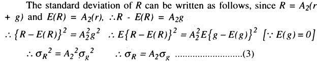
This shows that the standard deviation of R depends on the standard deviation of g and on the proportion invested in bonds. From equations (2) and (3), it can be seen that the proportion invested in bonds A₂ determines both E(R) = µ_R and the risk σ_R of the portfolio.

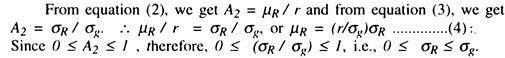
Equation (4) gives us a relation between µ_R and σ_R. This is the opportunity locus of the investor which shows the terms on which the investor can get higher expected return at the expense of assuming more risk. If we plot σ_R on the horizontal axis and µ_R on the vertical axis, we can get a straight line through the origin with slope (r/σ_g). In Fig. 5.3, the line OC₁ represents the opportunity locus when the current rate of interest is r₁. The slope of OC₁ is (r₁/σ_g).

If the rate of interest is r₂, the opportunity locus becomes OC₂ which is steeper than C₁ when r₂ > r₁. Since σ_R < σ_g, the lines OC₁ and OC₂ terminate at σg. Given the current rate of interest the opportunity locus is fixed. The opportunity locus gives the different opportunities open to an of the investor.

The preference pattern or utility function is represented by an indifference map. Let us assume that utility received by the investor, U, is a function of µ_R and σ_R, i.e., U = U (µ_R, σ_R). Indifference curves measure the level of utilities. The greater the utility level, the higher will be the indifference curve. The investor is indifferent between all combinations of (σ_R, µ_R) that lie on the same indifference curve (I). The slope of IC depends on the nature of the investor’s preference between return and risk.

The equilibrium solution is reached when the highest possible indifference curve is attained within the budget constraint. In Fig. 5.3, highest attainable indifference curve I₂ is reached at T₁ with the opportunity locus OC₂. At point T, σ_R < σ_g, which means σ_R < σ_g < 1 i.e., A₂ < 1. In this equilibrium point, individual holds both cash and bonds. Such an investor who holds some amounts of both the assets is called a diversifier.

The equilibrium may also be achieved at the corner point C₂ where µ_R = r₁ and σ_R= σ_g, as in Fig. 5 4. In this case, the highest indifference curve I₂ passes through the point C₂. At this point (C₂), σ_R= σ_g, σ_R‘/ σ_g = 1 or A₂ =1. In this case, the entire amount of wealth is held in the form of bonds.

Similarly, a corner equilibrium can also take place at O where σ_R = 0, i.e., A₂ = 0 and A₁ =1. In this case, the entire balance is held in cash. Such a solution can be shown in Fig. 5.5. The highest indifference curve is I₂ which passes through O and as this is in equilibrium the investor holds all cash and no bond. These corner solutions indicate that investors are non-diversifiers. 

Empirically, we find that most of the investors in the real world are diversifiers. Thus, the situation depicted in Fig. 5.3 may be taken as the standard case. Now let us see how in the standard case, the portfolio equilibrium changes with change in the current rate of interest. This is shown in Fig. 5.6. Suppose the current rate of interest is r₁. At r₁ the opportunity locus is OC₁ and it is tangent at T₁ with indifference curve I₁.

Now suppose the rate of interest increases to r₂. At r₂, the opportunity locus is C₂ and the point of tangency between I₂ and C₂ is at T₂ and so on. The locus of the successive points of tangency between ICs and opportunity loci is called the optimum portfolio curve. From the opportunity portfolio curve, we can see that as the interest rate increases, σ_R also increases where σ_R1, < σ_R2 < σ_R3. It follows from constant σ_g that σ_R1/σ_g < σ_R2/σ_g < σ_R3/σ_g. This means that as the rate of interest increases, so also the portfolio of bonds held increases. As A₂ increases, A₁ decreases.

Thus, as the interest rate increases so the proportion of wealth held in the form of cash decreases. This gives us an inverse relationship between the rate of interest and the demand for cash. So the portfolio balance approach can explain the downward sloping liquidity preference function.

It is also possible to have an optimum portfolio curve downward sloping which means that as the interest rate goes up, the proportion invested in bonds decreases. This is shown in Fig. 5.7 where σ_R2 < σ_R1, so that σ_R2/σ_g < σ_R1/σ_g. This means that A₂ decreases as the interest rate increases. Here A₁ increases as A₂ decreases. Thus, we get a direct relationship be­tween the rate of interest and the demand for cash. This ambiguity can be explained with the help of income and substitution effects of a change in the rate of interest.

The optimum portfolio curve is similar to price consumption curve. When we move along the price consump­tion curve, a price effect takes place which is the result of income and substitution effects. Similarly, the rate of interest can produce two such effects. For example, an increase in the rate of interest provides incentive to take more risk due to substitution effect which tends to increase A₂.

At the same time a higher interest rate increases the real income of the investor and gives him more security. This income effect will tend to reduce A₂. Thus, the income effect and substitution effect work in opposite directions. The net effect will depend on the relative strengths of these two effects.

If the income effect-is stronger than the substitution effect, we shall get a direct relationship between the rate of interest and the demand for cash, as shown in Fig. 5.7. On the other hand, if the substitution effect is stronger than the income effect, we shall get an inverse relationship between the rate of interest and the demand for cash, as shown in Fig. 5.6.

The portfolio balance approach has the great merit that it can explain the inverse relationship between the demand for cash and the rate of interest without assuming inelasticity of expectations of future rates of interest. It also provides an explanation of why rational individuals hold diversified portfolios containing both cash and bonds. This approach provides a logically more satisfactory foundation for the Keynesian liquidity preference theory. It is not difficult to extend this theory where there are more than two assets.

14. Milton Friedman Modern Quantity Theory:

Milton Friedman restated the quantity theory as a theory of the demand for money, and this ‘Modern Quantity Theory’ has become the basis of view put forward by monetarists. In this theory, money is seen as just one of a number of ways in which wealth can be held, along with all other human and non-human wealth.

Since money is seen as just one of the ways in which wealth can be held, Friedman sees the real demand for money (M_D/P) as depending on total wealth (W), the-expected rates of return on the various forms of wealth (r), the ratio of human to non-human wealth (ω) and society’s tastes and preferences (T). We can write functionally as M_D/P = f (W, r, ω, T). Consider each of the independent variables in turn.

Total Wealth (W):

The demand for money will be directly related to total wealth so long as money is regarded as a ‘normal good’ by wealth-holders. Thus, as total wealth increases, the desire to hold money will also increase.

Expected Rates of Return on Wealth (R):

Since the rates of return on bonds and equities are the opportunity cost of holding money, we can expect an inverse relationship between these expected rates of return and the demand for money. Note that, in addition to the various rates of interest, the expected rate of inflation should also be taken into account. The higher the rate of inflation, the greater is the negative return from holding money and the more attractive are the interest-bearing assets. Thus, there is also an inverse rela­tionship between the rate of inflation and the real demand for money.

The Ratio of Human Wealth to Non-human Wealth (W):

This variable is included by Friedman because human wealth is very illiquid. It cannot be sold and individuals have a limited ability to transfer non-human wealth into human wealth. The higher the ω ratio, the greater will be the demand for money in order to compensate for the limited marketability of such wealth

Tastes and preferences (T):

Friedman argues that the demand for money is also a function of a number factors which are likely to influence wealth holders’ tastes and preferences for money.

The fundamental problem with this demand for money function is to find a method of measuring total wealth. According to Friedman, the permanent income (Y_p) may provide a proxy variable. This is a long-run measure of income which can be thought of as the present value of the expected flow of income from the stock of human and non-human wealth over a long period of time.

It is normally estimated as an average of past, present and expected future incomes. Incorporating this into the function, and assuming that T and ω are constant especially in the short-run, we can write as: M_D/P = f (Y_p, r) which is not very different from Keynesian liquidity-preference function, L = f(Y, r). There are, however, two crucial differences.

First, in the Keynesian function — where money is a close substitute for bonds only — the demand for money is interest-elastic, because if the rate of return from holding bonds changes, wealth holders are unlikely to react in any other way than chancing their money holdings; but in Friedman’s money demand function money is likely to exhibit low interest-elasticity. Secondly, the Keynesian function includes current (Y) income only, whereas Friedman uses permanent income (Y_p) as a proxy variable for total wealth.

The precautionary motive is just as important as a motive for holding money as the other. In transaction demand for money, we focussed on transaction costs and ignored uncertainty. Here we concentrate on the demand for money that arises from uncertainty about the payments they might have to make.

Suppose that people do not know precisely what payments they will be receiving in the next few weeks and what they will have to make. The person might need to take a cab in the rain, or have to pay for a prescription. If they do not have to pay, they will incur a loss. Let us denote the loss incurred for a shortage of cash by £q.

The more money people hold, the less likely they are to incur the costs of illiquidity. But the more money people hold, the more interest they will have to forgo. We are back to a trade-off situation similar to that examined in relation to the transactions demand. Somewhere between holding so little cash that one will have to forgo some purchase and holding lots of money so that there is little chance of not being able to make any payment, there must thus be an optimal amount of precautionary balances to hold.

To determine the optimal amount of money to hold, we compare the marginal cost (M_C) of increasing money holding by £1 with the expected marginal benefit (M_B) of doing so. The (M_c) is the interest forgone or r which is shown in Fig. 5.8. The M_B of increasing money holding arises from the lower expected costs of illiquidity. Increased precautionary balances from zero has a large M_B, since that takes care of small, unexpected disbursements that are likely to occur.

As we increase cash balances further, we continue to reduce the probability of illiquidity at a decreasing rate. Thus, the M_B of additional cash is a decreasing function of cash holdings, as shown by the M_B curve in Fig. 5.8.

The optimal level of precautionary demand is reached at M* where M_C = M_B. It is clear from Fig. 5.8 that precautionary balances will be larger when the interest rate is lower. A reduction in the interest rate to r₁ shifts the MC to Mc and increases M* to M*₁. The lower cost of holding money makes it profitable to insure more heavily against the costs of illiquidity. An increase in uncertainty leads to increase in money holdings because it shifts up the M_B to M’_B and M* to M*₂ .Finally, the lower the costs of illiquidity, q, the lower the money demand.

The precautionary demand-depends on: the alternative costs in terms of interest forgone, the cost of illiquidity, and the degree of uncertainty that determines the probability of illiquidity.

15. Karl Marx’s Classical Theory of Full-Employment:

Karl Marx gave the name ‘Classical Economics’ to the writings of Adam Smith, David Ricardo and their followers who investigated relations of production in bourgeois society. Subsequent economists, like Marshall, Edgeworth, Pigou and their followers who believe in Say’s law of markets, are also called classical economists. Say’s law states that the supply creates its own demand and there is no possibility of general over-production.

The classical economists believe that in a competitive capitalist economy there exists an automatic mechanism which brings about full employment. This automatic mechanism is known as ‘invisible hand’ and impersonal market forces emanating from individual behaviour patterns are governed by self-interest.

The classical model of income and employment determination is divided into four markets: the money market, the commodity market, the bond market and the labour market. However, following Walrasian law, the commodity market is dropped and the equilibrium conditions in three markets — the labour market, the money market and the bond market — are considered. In each market, there exists a demand function, a supply function and equilibrium condition. Thus, the classical model can be represented with the help of certain equations.

We start our analysis with the labour market of the economy. It is assumed that there exists an aggregate production function, the demand function for labour and the supply function of labour. The aggregate production function describes the relationship between real income (Y) and the level of employment (N), given the capital stock Y = f (N, K₀)………… (1) where Y is output, N is employment and K₀ is the given capital stock. We assume that the marginal productivity of labour is positive but follows a diminishing marginal product of labour i.e., dY/dN >o and d²Y/dN² <0. Profit-maximisation under perfect competition leads to production of output at the point of equality between the real wage rate and the marginal product of labour.

The quantity of output to be produced determines the number of people to be employed. Alternatively, given the money wage rate, profit-maximising employment is directly determined at the point of equality between the money wage rate and the value of the marginal product, provided that it is falling at the level of employment. The value of marginal product is the marginal product multiplied by the price of the product.

The profit-maximising condition can be written as w = P. dY/dN where W is the money wage rate and P is the price level or W/P = dY/dN …….. (2) that is, the real wage rate should be equal to the marginal physical product of labour (MPP of L). If we plot the level of employment on the horizontal axis and the real wage rate on the vertical axis, the marginal product of labour curve will give us the labour demand curve. It gives us the amount of labour demand at different real wage rates.

Thus, we get the inverse relationship between the real wage rate and the demand for labour. Now we consider the supply curve of labour. It is assumed by the classical economists that money wages and prices are flexible both in the upward and in the downward directions. The supply of labour is assumed to be a direct function of the real wage rate which means that the real wage rate increases so the supply of labour also increases. The classical labour supply function can be written as: N = N (W/P)………. (3) such that dN/ d(W/p) > 0.

Thus we get the following three equations for the labour market:

1) Y= f(N, K₀)

2) dY/dN = W/P

3) N = N (W/P)

From these three equations, we can solve for three unknowns: Y, N and W/P, i.e., the level of income, level of employment and real wage rate can be determined from the above three equations. Now consider Fig. 7.1 where the upper graph shows the aggregate labour market at a real wage rate of (W/P) and the level of employment equals to ON_f.

At the intersection of the downward sloping labour demand curve and the upward sloping labour supply curve, the equilibrium real wage rate and the equilibrium level of employment is determined. Once we know the equilibrium level of employment, it is easy to get the equilibrium level of income from the aggregate production function in the lower graph in Fig. 7.1. The equilibrium level of employment N_f the equilibrium real wage rate (W/P) and the equilibrium level of output Y_f are given in Fig. 7.1. The classical economists called this equilibrium the ‘full employment’ level.

According to them, any unemployment that existed at the wage rate (W/P)_f must be due to frictions or restrictive practices in the economy or must be voluntary. At the real wage rate (W/P)_f , those who are willing to work at the going wage rate would find jobs. If the real wage rate is greater than (W/P)_f labour supply will be greater than labour demand and unemployment will prevail. There is no problem in the classical model where money wages are flexible.

If there is unemployment, money wages will fall because of competition among workers. As money wages fall, the employment of more labour becomes profitable. More workers will be demanded and more employment will be created. As a consequence, the supply of output will also increase. The additional output can only be disposed off if the price level falls.

Thus, if the price level decreases in the same proportion, the real wage rate will remain unchanged and the incentive to employ more workers will not be present. Hence it is necessary that the classical model requires that the price level must fall in lower proportion than money wage rate.

In other words, so long as there is unemployment in the economy, the real wage rate will fall, the supply of labour will decrease and the demand for labour will increase until full employment is reached. Thus, perfect flexibility of money wages and prices will automatically achieve full employment in the labour market. There cannot be any question of underemployment equilibrium in the classical model.

Now, let us consider the determination of interest rate in the classical model. For this we need to consider the bond market of the economy. The classical model assumes that whatever is saved is lent and whatever is borrowed is invested. Households save to buy bonds and firms finance their investment by selling bonds to the households.

Thus, saving is connected with the demand for bonds and investment is connected with the supply of bonds. Since the rate of interest is determined by the supply of and the demand for loans, it is known as loanable fund theory of interest rate determination. According to classical economists, the interest rate is determined by the equality of saving and investment — both of which are functions of rate of interest.

We can write the saving function as: (4) S = S(r) where S'(r) > 0. It is assumed that investment is an inverse function of the rate of interest, which means as the rate of interest rises, investment decreases. (5) I = I(r) such that I'(r) < 0. Equilibrium condition requires that (6) S = I. Note that the determination of the rate of interest is in no way related with the determination of the equilibrium values of the other variables in the system. The complete classical model requires the equations of the money market.

In the money market we have one money demand curve, one money supply curve and one equilibrium condition. Classical economists only considered the transactions demand for money. The demand for money is thus a function of the level of income only and not a function of the rate of interest.

It can be assumed that the demand for money is a constant fraction of the money national income, i.e. (7) M_d = kPY, where M_d is the demand for money, Y is the real output, P is the price level and k is a constant fraction. On the supply side it is assumed that the supply of money is exogenously given, M₀ i.e. (8) M_s = M₀. Equilibrium condition requires M_d = M_s. The money market equilibrium condition can be written as (9) M₀ = kPY. But we already know Y from equations (1) to (3).

Thus we can find P from the equilibrium condition of the money market i.e. from equation (9). We have already known the equilibrium value of W/P. If we know P we can determine W. Therefore, the money wage rate can also be determined. Since M₀ and k are constants, equation (9) can be written as PY = M₀/k = constant.

This shows that as Y increases P must decrease since PY is a constant.

The equation py = M₀/k is presented in Fig. 7.2.

The complete classical model contains the following 9 equations:

1) Y  = f(N, K₀)

2) dY/dN = W/P

3) N = N(W/P)

4) S = S(r)

5) I = I(r)

6) S = I

7) M_d = kPY

8) M_s = M₀

9) M_d = M_s

There are also 9 variables in the model: Y, N, W, P, M_d, M_s, S, I, r. Thus, the system is determinate. It may also be noted that the system is decomposable. We can solve equations (1) to (3) for 3 variables: Y, N, W/P. Once Y is known the equations (7) to (9) determine P. Equations (4) to (6) determine the rate of interest independently. Graphically the complete classical model can be represented in Fig. 7.3. In part I, we have drawn the labour demand curve and the labour supply curve.

In part II, we determine the equilibrium level of output. In part III, we have drawn the rectangular hyperbola and, in part IV, we have drawn a straight line through the origin with the slope (W/P)_f. The equilibrium level of employment and the equilibrium real wage rate is determined in part I of the Fig. 7.3. Part II-determines the equilibrium level of output. Given the level of output in part II, part III determines the equilibrium price level and the part IV determines the equilibrium money wage rate.

In part V, equilibrium rate of interest is determined. Note that parts I to IV are linked with one another but part V is not connected with them. This shows that the determination of the equilibrium rate of interest is not connected with the determination of the equilibrium values of other variables. This means that any change in the savings or investment function will affect only the interest rate and not the other variables.

For example, if the investment function shifts in the downward direction and the saving function remains unchanged, then only the equilibrium rate of interest will fall to r ’. But it will have no impact on employment, money wage rate, price level and real income.

In the classical system, there are two parts — the real part of the system and the monetary part. The real variables such as the real wage rate, the level of output and employment are determined in the real sector while the monetary variables such as the price level and money wage rate are determined in the monetary part.

 16. Wicksell’s Demand-Pull Theory of Inflation:

The earliest attempt was made by classical economists to explain inflation with the help of the quantity theory of money. According to this theory, the price level depends directly and proportionately on the quantity of money. Inflation occurs when the quantity of money increases. The rate of inflation depends on the rate of money supply.

The quantity theory, however, could not explain the mechanism through which price level will rise as a result of the rise in money supply. It was Wicksell who analysed the mechanism by which an increase in money would lead to an increase in the price level.

He pointed out that an increase in money supply increases the aggregate demand in the economy. Wicksell’s theory states that, when money supply increases, the market rate of interest falls below the natural rate and this will induce investors and consumers to spend more in the economy. As a result, the aggregate demand will increase-which will increase the price level— assuming that aggregate supply will remain constant at full employment level. The price level will go on increasing, so long as the market rate of interest is below the natural rate.

When money supply will stop increasing, the market rate of interest will rise and become equal to the natural rate and the inflationary pressure will be halted with it. Wicksell realised that the rise in the price level itself would not reduce aggregate demand, because, after a time lag, money incomes would rise in proportion to prices, leaving consumers and investors to compete for the limited supply of goods.

Keynesian theory of inflation is nothing more than a modification and generalisation of Wicksell’s theory of inflation. Suppose, there is already full employment in the economy, and investment demand increases. This means that, total demand for goods and services is greater than the available supply. Thus, prices are bid up.

Since consumer demand depends on real income which is not reduced by rising prices because the sale at higher prices creates an equivalent rise in money wages without eliminating excess demand. Thus, Keynes broke the dose link between the quantity of money and the level of aggregate demand associated with classical-economists. According to Keynes, there may be some inflation in the economy even with a constant money supply. In a situation of constant money supply, an increased price level would raise the transaction demand for money and, thus, push up interest rate, which would reduce investment demand.

The decreased investment demand will moderate the inflationary pressure, but is unlikely to eliminate it. The reason is that the rise in interest rate will free some money from speculative demand to meet the added transaction demand. Only at zero speculative demand this would correspond to Wicksell’s theory.

There is, thus, a significant difference between Wicksell’s and Keynes’ theory of inflation. For the former any increase in the supply of money is inflationary. For the latter, the rise in prices may occur even without any increase in the supply of money.

Again, an increase in the supply of money may not have any impact on prices in the Keynesian System, especially if the economy starts from a position of unemployment. Despite these differences, both the theories explain inflation as arising from an excess of aggregate demand over the full employment aggregate supply.

The Keynesian theory of inflation is normally explained with the help of “inflationary gap” which is defined as an excess of aggregate demand over aggregate supply at full employment. Fig. 16.9 explains the condition of disequilibrium that exists in output market as a result of the emergence of the inflationary gap. In the vertical axis, we measure the total expenditure (E = C + I + G + X – M) and in the horizontal axis, we measure real income. Let Y₀ be the value of the full employment output, which has been assumed to be a fixed quantity. If C + I + G + NX is the aggregate demand curve, Y₀ = C + I + G + NX at A and, then, the price level is in equilibrium.

If, for some reasons, the aggregate expenditure curve shifts to C’ + I’+ G’ + NX’, an inflationary gap appears in the output market. The size of the inflationary gap is AB which measures the excess of the aggregate demand over the value of the full employment output; it is given by C’ + I’ + G’ + NX’ – Y₀. The money value of the real output will be in equilibrium at Y_m.

This can be done through the rise in the price level, as the real output is constant at full employment. So long the inflationary gap exists the price level will go on increasing. Inflation goes on without limit unless the inflationary gap is eliminated by actions of fiscal and monetary authorities or by the indirect effect of inflation on real demand. If aggregate demand is less than aggregate supply at full-employment then we have the deflationary gap. When there is a deflationary gap, the economy will settle at a less than full employment situation.

We now examine the indirect effects of the existence of inflationary gap on the components of demand and see whether the inflationary gap can automatically be eliminated as a result of the operation of these indirect effects.

First, if money supply remains constant the rate of interest will increase because the price increase will reduce the real money supply. As the rate of interest increases, the investment demand will fall and the aggregate demand will be reduced, thereby eliminating a part of the inflationary gap.

Second, as a result of the operation of the Pigou effect, an increase in the price level will reduce the real value of the given supply of money, which will reduce the aggregate real consumption expenditure thus shifting the consumption function— and, consequently, the aggregate demand function—in a downward direction.

Third, indirect effect of the price increase would be to redistribute income against fixed income groups (i.e. between wages and profits). If the MPC of the fixed income groups is assumed higher than the average of the economy, such redistribution will reduce aggregate consumption expenditure.

Fourth effect is that as the tax collection rises faster than prices (especially in the case of income tax) disposable income will fall—which will also reduce consumption expenditure.

Fifth effect of higher domestic price will tend to discourage exports and encourage imports which will reduce net exports (X-M). However, Keynes was of the opinion that neither of these indirect effects would be able to eliminate the inflationary gap.

Keynesian theory of inflation suffers from the following limitations. This is a static theory, which does not determine the rate of inflation. This limitation can be removed by dynamising it by assuming that the rate of inflation is proportional to the length of the inflationary gap.

This theory has considered excess demand in the commodity market only. If there is excess demand in the factor market inflation may develop from that market. This possibility has not been considered by Keynes at all. This limitation has been removed by Hansen, who has introduced both goods and factor gaps in the analysis of inflation.

The Keynesian theory assumed that inflation arises only after full employment is reached So long full employment is not reached, there is no possibility of price increases. But when full employment is reached, the supply of com­modity remains stationary and only the price level can increase. But, in reality, the inflation can begin even in a period of unemployment as we have seen in the 1970s and 1980s. Keynes also ignored the cost push inflation.

Even when there is unemployment in the labour market, the wage rate may increase due to trade union pressure. If the productivity of labour does not increase with wage increases, unit cost of production will increase. This will push-­up prices.

17. Marxist Theory of Economic Growth:

Marx rejected some principal features of the Classical theory of economic growth and offered his own theory within a socio-historical framework in which economic forces play a major role. In Marxist theory, the law of diminishing returns has been discarded because Marx believed that the Classical theory of Stationary State was actually a creation of human actions rather than the end product of a natural, immutable law. For a similar reason, Marx also castigated the Malthusian theory of Population.

Marx looked at economic development from a social and historical stand­point. Each stage of economic growth was regarded as the product of Hegelian dialectics of a game of contradictions where a thesis created its anti-thesis and the conflict between the two produced a synthesis. Marx emphasised that, with capitalism, social relations of production are much more important than an exchange relations between goods.

The social character of labour has been stressed in particular. Marx argued that labour productivity ‘is a gift, not of nature, but of history embracing thousands of centuries’. However, the Marxist concept of relations of production is rather vague. It has been interpreted as an ‘organic whole’ characterized by labour organisation and skill, the standing of labour in society, technological and scientific knowledge and its use in a certain environment.

In the Marxist analysis, these ‘relations of production’ determine the socio-cultural set-up of a society. Marx believed that capitalism would not end up in a quiet classical ‘stationary’ state; rather, it would break up with a ‘bang’ ‘when the expropriators are expropriated’. Here we shall only analyse the economic views in the Marxist theory.

The Marxist model of economic growth depends on some major dynamic ‘laws’:

(1) The law of capital accumulation, which says that the prime desire of the capitalists is to accumulate more and more capital.

(2) The law of falling tendency of the rate of profit which plays a crucial role in the breakdown of the capitalist system.

(3) The law of increasing centralisation and concentration of capital, which tells us that, with the growth of capitalism, cut-throat competition among capitalists will lead to the annihilation of the smaller firms by bigger ones, which will lead to the growth of monopoly and concentration of economic power.

(4) The law of increasing ‘pauperization’ which implies the growth of the misery of the working class with the advancement of capitalism, reflected in wages being tied to the subsistence level coupled with a rise in the proportion of unemployed people — or, what Marx called the ‘industrial reserved army of labour’— made possible by the substitution of capital for labour in the process of technical change.

The simultaneous working of these laws would generate contradictory forces, which would eventually sharpen the class conflict between capitalists and workers or between ‘haves’ and ‘have-not’s’. Capitalism would face a violent death in the final confrontation, when the expropriators would be expropriated. Hence, Marx gave the clarion call: ‘workers of the world unite’, as they have nothing to lose except their ‘chain’ and ‘the whole world to conquer’.

The Marxist notion of the falling tendency of the rate of profit plays a crucial role in the whole process of change and can now be illustrated. According to Marx, the value of a commodity (W) is given by the sum of ‘constant capital’ (c) + the ‘variable capital’ (q) + the ‘surplus value’ (s).

If the working day consists of 8 hours and only 4 hours are required to produce a commodity for subsistence then for the remaining 4 hours, the worker is producing a surplus value, which is expropriated by the capitalists. More formally, W = c + q + s and X = s/q where x is the rate of surplus value or the rate of ‘exploitation’. Thus, in the above example,

4 hrs/4 hrs = 100% = X

The rate of profit (P) in the Marxian analysis is given by:

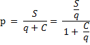
Let S/q = X, i.e. the rate of exploitation, and c/q = J or the ‘organic composition of capital’. Then we have p = X/1 + J .Now, it is clear that, if X remained constant, P and J would be inversely correlated. A rise in J would take place as capitalism developed with continuous accumulation. Also, capitalists would substitute capital for labour whenever wages tended to rise above the subsistence level to maintain their rate of profit.

The process would lead to higher unemployment among the working class and sharpen the polarization of forces. On the other hand, the crisis of capitalism would be reflected in the periodic fluctuations of growth and a falling tendency of the rate of profit, which would lead to cut-throat competition among the capitalists which, in turn, would lead to monopoly. Eventually, the conflict between the ‘immiserized proletarians’ and the capitalists would toll the death-knell of capitalism.

It is interesting to observe that the falling tendency of the rate of profit may not always be seen within an economic system. This can easily be demonstrated within the Marxist model. We have P = X/1 + J. Differentiating P with respect to time we get:

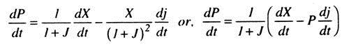
Note that the profit rate will rise if the rate of exploitation rises more rapidly than the organic composition of capital. Even if the rise in the organic composition of capital is higher than that of the rate of exploitation, whether or not profit will fall depends on the difference between dx/dt and the product of profit rate and dj/dt.

For profit rate to fall, Pdj/dt (which is negative) must be greater than dx/dt. But a fixed rate of exploitation and an increase in capital intensity may not go together because a rise in organic composition of capital would raise labour productivity which would either raise the rate of exploitation or raise real wages. Inevitably, the internal consistency of the Marxist model has been questioned.

Further, a rise in the organic composition of capital could increase the rate of profit with an increase in productivity and a change in technology. Under such circumstances, the intensity of competition among capitalists declines. Technical progress may be neutral or even labour-using. Thus, the rise in the industrial reserve army of labour and a fall in the wage share in national income may not occur.

Other criticisms usually leveled against Marxist model may also be briefly mentioned. It is contended that Marx’s correlation between the growth of the average firm size and an increase in the degree of concentration need not always happen. However, the proportion of unemployment has increased in recent decades.

Empirically, wage share of national income in most developed economies remained fairly constant for a long lime and this phenomenon seems to have weakened the Marxist law of increasing pauperization. On the other hand, the Marxist prediction about the increasing concentration and centralisation of capital is not rejected. However, the rise in the output-capital ratios in developed economies probably reflects the growth of both accumulation and real wages, a phenomenon which Marx probably did not envisage within the strict framework of his analysis.

18. Rostow’s ‘Stage’ Theory of Development:

This theory states that the transition of an economy from being less developed to developed is possible through a series of steps. The most important of these is the so-called ‘take off stage when resistance to change in traditional values and, in the social, political and economic institutions of an underdeveloped economy is finally overcome and modern industries begin to expand. The theory may be criticised for viewing development as simply a matter of higher saving and investment ratios.

Saving and Investment:

Physical capital has always been at the centre of economic development. In order to invest, the country must save or, else, must have access to foreign saving through loans and aid. If domestic saving is the prerequisite for capital accumulation, then attention must focus on policies to promote saving.

Saving does depend on the availability of saving instruments — a banking system that offers convenient deposit services. There is evidence that extreme financial instability interferes with saving. When the return on saving becomes negative one of three things happens: households reduce their savings or they shift their saving abroad or they accumulate their saving in unproductive assets, such as gold. The financial environment for saving is thus an important factor in channeling saving from households to investing firms.

In addition to the private sector, the government affects national savings through its budgetary policies. It can also draw foreign savings to finance investment. A developing economy can tap foreign savings in three ways. One possibility is that, foreign firms invest directly in a country. The second way is that a country can tap foreign resources by borrowing in the world capital market or from institutions, such as the World Bank. Third possibility is that a country may receive foreign aid from industrialised countries.

The importance of these three sources of external saving has varied over time and between countries. But, there is no doubt that external saving can supplement domestic saving as it always has done. Of course, foreign saving is all the more important the lower the per capita income.

The amount of saving, whatever, may be its source, determines how much investment will take place in a country. But the productivity of investment may vary widely. The larger differences in productivity of investment across countries focuses attention on development policies and strategies that affect the efficiency of resource utilisation.

19. Alfred Marshall and A.C. Pigou’s Quantity Theory:

The Cambridge economists—like Alfred Marshall and A. C. Pigou—presented an alter­native to Fisher’s version of Quantity Theory. They have attempted to establish that the Quantity Theory of Money is a theory of demand for money (or liquidity preference). The Cambridge version of the Quantity Theory of Money is now presented.

Formally, the Cambridge equation is identical with the income version of Fisher’s equation:

M = kPY, where k = 1/V in the Fisher’s equation.

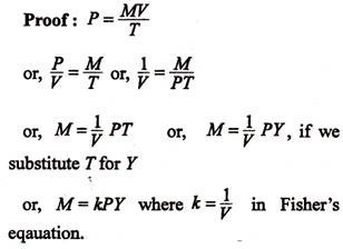
Here 1/V = M/PT measures the amount of money required per unit of transactions and its inverse V measures the rate of turnover or each unit of money per period.

So if k and Y remain constant, P is directly proportional to the initial quantity of money (M).

Criticisms:

1. The chain of causation:

Critics argued that all the factors in the equation of exchange are variables and statistical studies have shown that they are interrelated. Moreover, the line of causation is not always from M (money supply) to P (the price level). It may be from V to P. A change in the rate of spending, all the other factors remaining the same, will result in a change in prices just as surely as would a change in the Quantity Theory of money, other things remaining the same.

Or a change in T, other things remaining the same, will cause a change in prices. So it is difficult to accept the theory that changes in the quantity of money are always the causes in the price level. Studies have shown that the price level cannot be easily and quickly controlled by changing the amount of money and credit available for the purchase of goods and services.

It may also be said that, under certain circumstances, an increase in the quantity of money will not produce any change in the price level. Keynes has pointed out that the Quantity Theory is inapplicable to a country which has unemployed resources (capital and labour not in use).

In such a country, creation of more money will lead to more employment and higher production (larger supply of goods) and no change in the price level. Prices will change in proportion to money supply only when there is no scope for increasing production, i.e., when there are no unemployed resources in the economy.

2. There are inactive balances:

Under Fisher’s formula, the price level depends upon the total quantity of money. But it is only a part of the total quantity of money which influences prices. There always exist inactive balances (hoards) which exert no pressure at all on the prices of goods and services. This is clearly seen during depressions.

3. Simultaneous changes:

The Quantity liquation cannot be used for analysing the effects, of changes in M, or T, on the price level except on the ceteris paribus assumption, “other things remaining constant.” But in the case of monetary variables such an assumption cannot be made. When M changes, T and V both change. When T changes, M, and V change. The net effect on the price level of a change in any of the variables of the quantity equation depends on how the other variables are simultaneously changed.

4. The process of change:

Theory does not show the process through which changes in the amount of money affect the price level. Keynes put great emphasis on this point.

He observed that:

“The fundamental problem of monetary theory is not merely to establish identities or statistical relation but to treat the problem dynamically, analysing the different ele­ments involved in such a manner as to exhibit the causal processes by which the price-level is determined and the method of transition from one equilibrium to another.”

5. The assumption of full employment:

So increase in the quantity of money does not always increase prices. If there are unem­ployed resources, increase of money increases employment and not prices. As Keynes points out, the Quantity Theory is based on the assumption of Full Employment.

6. The value of money determines the quan­tity of money:

According to Quantity Theory, an increase in the supply of goods or it will cause a fall in the price level P. Monetary and banking practices, increases in the supply of goods always leads to an increase in the supply of money (through creation of credit and otherwise). M therefore, depends on T; they are not independent variables. If this view is correct, the value of money is not deter­mined by its quantity; on the contrary it is the value of money which determines its quan­tity.

7. Non-monetary factors:

Prices may change and the value of money vary for reasons entirely unconnected with the quantity of money.

Some examples are given below:

(i) Changes in the level of efficiency wages may change costs of production and affect prices.

(ii) If increase of output occurs under con­ditions of diminishing returns, marginal costs will rise and prices will rise. Similarly, prices will fall if production increases under con­ditions of increasing returns.

(iii) Increase and decrease of monopoly power will, respectively, increase and decrease prices.

(iv) Prices are affected by variations in effective demand or expenditure. Consumption expenditure and investment expenditure both vary—as also the proportion between them.

8. Misleading emphasis:

Finally, according to Crowther the Quantity Theory puts a mis­leading emphasis on the importance of the quantity of money as the cause of price changes and pays too much attention on the level of prices. In the short rim these principles of the Quantity Theory are not in accord with facts. In actual life the price level and volume of production move up and down in a cyclical pattern.

The Quantity Theory draws pointed attention to one important factor which causes price change, viz., the quantity of money. It is admitted that the quantity formula “hides many links in the chain of causation”, but it is undisputed that the formula gives us a rough and ready method of determining the effects of changes in the quantity of money and certain other factors influencing the price level.

From the above discussion it is clear that the Quantity Theory is inadequate and defec­tive. It has, however, certain merits. Generally, we find that when money supply increases, the price level rises. For example, during 1939-45 in India there was a large increase in the volume of notes and bank advances and the price level rose very fast. Hence, there is some relationship between the quantity of money and the value of money. The Quantity Theory states the relationship not with absolute correctness but only approximately.

Dr. Milton Friedman (the 1976 Nobel Prize winner) believes that the quantity theory of money is true in its simple or cured form, i.e., price (P) varies with quantity of money (M). He believes that there is a proportionality between the quantity of money and the general price level in an economy.

20. W.J.L Ryan Theory of Profit:

A firm under perfect market condition maximises profit in the short run when price becomes equal to marginal cost for its product. But, in the long run, due to the unbridled free entry, profit is competed away and the firm earns only normal profit, that is, wages of routine management which is included in the cost of production.

In the language of W. J .L. Ryan: “Profits are absent in the state of perfect competition because each entrepreneur has equal opportunities and equal capacities to exploit them.” But, since perfect competition refers to an unreal situation, a brief sketch of profit theory may begin with its elimination. For example, we may mention monopoly revenue although economic usage calls it profit.

Modern business revenue devices may make it possible to prolong the temporary gains of a quasi- monopolistic firm accruing from successful innovations. Moreover, other factor like barriers to entry, product differentiation, etc., may result in the existence of pure profit, both in the short run and in the long run under imperfect competition.

Many people regard profit a necessary evil but it is the earning of monopoly.

A. P. Lerner has developed a measure conveniently called “degree of monopoly power” which is defined as the excess of price over marginal cost, divided by the original price. In symbol,

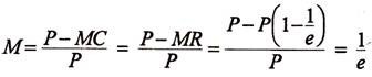
Where M stands for monopoly profit, and other symbols have their usual meanings.

Thus, the more inelastic the demand for a commodity is, the greater will be the scope of exploitation by the monopolist and the greater will thus be the volume of monopoly profit. As Lowes and Sparkes put it: “Profits accrue to companies as a result of the monopoly power which they possess in their markets, which allows them to raise price by restricting output.”

According to Paul Samuelson profit occurs due to ‘contrived’ or artificial scarcities — a surplus return.