Economic Models: 10 Economic Models Formulated by Eminent Economists

Read this article to learn about some of the most important economic models formulated by eminent economist:

(1) Models of Oligopoly, (2) Baumol-Tobin Model of Cash-Management, (3) Keynesian Model of Income Determination, (4) Complete Keynesian Model of Money Supply, (5) Mundell-Fleming Model, and Others.

Model # 1. Models of Oligopoly:

Non-Collusive Oligopoly:

Cournot Model:

Oligopoly is a few sellers-market. Duopoly—a two firm model—is an extreme form of oligopoly. Duopoly model was first popularised by the French economist Augustin Cournot in 1838. Cournot assumes that there are two firms—1 and 2—that produce homogeneous goods, say X, and know the market demand curve. Both firms have the same cost functions. It is also assumed that each firm takes its rivals/competitors into account and assumes that its competitor is doing likewise.

The basic element of the Cournot model is that each firm treats its rival’s output as constant at the existing level and then decides its own output level so as to maximise profit. Thus, the output decision of one firm will depend on how much the rival is expected to produce.

Let us first consider the output decision of firm 1. Firm 1 thinks that firm 2 will produce nothing. Then firm 1 s effective perceived demand curve can be thought of as the market demand curve. This is shown by the curve D₁ (0) in panel (a) of Fig. 9.16. Thus, its profit-maximising output is 150, determined by MR (0) and constant MC curves. If firm 1 thinks that firm 2 will produce 100 units, then its demand curve would be the market demand curve shifted to the left by 100 units.

Thus to maximise profit, firm 1 would now produce 100 units—determined by the intersection of MC and MR(100) curves (shown in panel b). Now suppose firm 1 thinks that firm 2 will produce 150 units. Then firm l’s demand curve is the market demand curve shifted to the left by 150 units. It is labeled D₁(150) and the corresponding MR curve is MR(150). Profit- maximizing output of firm 1 would now be 75 units, the point where MC = MR(150) (shown in panel c).

Thus, we can summarise: If firm 1 thinks that firm 2 will produce nothing then it will produce 150 units (panel a); if it thinks that firm 2 will produce 100 units, it will also produce 100 units (panel b); if it thinks that firm 2 will produce 150 units, it will produce 75 units (panel c). Thus, we have three points in this figure. These points are labeled A, B and C in Fig. 9.17. The result thus obtained is called firm 1’s reaction curve. This is so called because profit-maximising output decisions of one firm is a function of other firm’s output.

In Fig. 9.17, we have drawn firm 1’s and 2’s reaction curves. Firm 1’s reaction curve ABCD shows how much it will produce as a function of how much it thinks firm 2 will produce. Likewise, firm 2’s reaction curve NBET shows its output as a function of how much it thinks firm 1 will produce. Equilibrium occurs at point B where the two reaction curves intersect each other.

Both firms would now produce 100 units of output. To see why B is the equilibrium point, let us consider point D on firm’s l’s reaction curve. Corresponding to this point, firm 1 would produce 50 units while firm 2 would produce 200 units. But firm 2’s reaction curve says that it would produce at point E (a lower output than 200 units) if it believes that firm 1 would produce just 50 units.

This cannot be equilibrium. “In equilibrium, each firm sets output according to its own reaction curve, so the equilibrium output levels are found at the intersection of the two reaction curves; we call the resulting set of output levels a Cournot equilibrium”.

Stackelbers Model: First Mover Advantage:

In the Cournot model we assume that the duopolists make their output decisions at the same time. Now we want to examine the advantage of the first mover. There are two questions of interest in this situation. First, is it advantageous to go first? Second, what is the resulting equilibrium?

Again we assume that the market demand curve is given by P = 30 – Q, where Q is total output and the MC of both firms is zero. Suppose, Firm 1 sets its output first and then Firm 2 makes its output decision. In setting output, Firm 1 must, therefore, consider the reaction of Firm 2. This is different from the Cournot model in which neither firm has the opportunity to react.

Let us start with Firm 2; because it makes its output decision after Firm 1, it takes Firm l’s output as given. Thus, Firm 2’s profit-maximising output is given by its Cournot reaction curve, as we found before.

Firm 2’s Reaction Curve: Q₂ = 15 –1/2 Q₁…………….. (2)

Firm 1 chooses Q₁, its profit-maximising output, where its MR = MC = 0. Recall that Firm l’s total revenue is:

TR₁ =PQ₁ = 30Q₁ – Q₁²– Q₂Q₁…………… (3)

Since TR₁ depends on Q₂, Firm 1 anticipates how much Firm 2 will produce. Firm 1 knows that Firm 2 will choose Q₂ according to its reaction curve given in equation (2).

Substituting equation (2) for Q₂ into equation (3), we find Firm 1’s TR₁ as: TR₁ = 30Q₁, – Q₁² – (15 – 1/2 Q₁) Q₁ = 15Q₁ – 1/2 Q₁².

So, its MR₁ = 15 – Q₁. Then setting MR₁, = MC₁ = 0, we get Q₁ = 15. And from Firm 2’s reaction curve (2), we find Q₂ = 7.5. Firm 1 produces 15 units of output which is twice as much as Firm 2’s 7.5 units and, thus, Firm 1 will make twice as much profit. Going first gives Firm 1 an advantage. It seems disadvantageous to announce output first. Why, then, is going first a strategic advantage?

The reason is that announcing first creates a fait accompli, no matter what your competitor does, your output will remain unchanged and large. To maximise profit, your competitor must take your large output as given and set a low level of output for itself. This kind of “first mover advantage” occurs in many strategic situations, as we will see later.

The Cournot and Stackelberg models are alternative representations of oligopolistic behaviour. Which model would be more appropriate depends on the industry. For an industry composed of roughly equal strength competitors, none of whom have a strong operational advantage or leadership position, the Cournot model may be more appropriate, whereas, some industries are often dominated by a large firm that normally takes the lead of setting prices and new production levels. The Sport shoe industry is an example in point, with Nike as the leader. In such a situation, the Stackelberg model may be more appropriate.

Price Competition with Homogeneous Products — Bertrand Model:

Our assumption so far was that oligopolistic firms compete by setting quantities, but, we find many oligopolistic industries where competition occurs along price dimensions. For example, for Ford, Chrysler and GM, price is a main strategic variable, and each firm chooses its price with its competitors in mind. Here we can use the Nash Equilibrium concept to study price competition, first in an industry with homogeneous product, and then in an industry with product differentiation.

Again, French economist Joseph Bertrand developed this model where, like the Cournot model, firms produce a homogeneous product. Now, however, they choose prices rather than quantity, which can dramatically affect the outcome.

We know that Cournot Equilibrium for this duopoly, which results when both firms choose output simultaneously, is Q₁ = Q₂ = 8. We also know that the equilibrium market price is £14, so that each firm can make a profit of £88.

Now, suppose, these duopolists compete by simultaneously choosing a price instead of a quantity. What price will each firm choose, and how much profit will each earn? The answer is that, because the good is homogeneous, consumers will buy only from the lowest price-seller.

Thus, if the two firms charge different prices, the lowest-price seller will supply the entire market, and the higher-price firm will sell nothing. If both firms charge the same price, consumers would be indifferent as to which firm they buy from; we can, thus, assume that each firm would then supply half the market.

The Nash Equilibrium in this situation is the competitive outcome, i.e., both firms set price equal to MC: P₁ = P₂ = MC = £3. Then industry output is 27 units, of which each firm produces 13.5 units. Since P = MC, both firms have zero economic profit. This is a Nash Equilibrium because neither firm would have any incentive to change its price. Suppose Firm 1 raised its price. It would, then, lose all of its sales to Firm 2, and would, therefore, be worse-off. Instead, if it lowered its price, it would capture the entire market, but it would still be worse-off because it would lose money on every unit it produced. Hence, Firm 1 has no incentive to deviate, it is doing the best it can, given what its competitor is doing.

A Nash Equilibrium cannot be at a price higher than the competitive price, because, in this situation, if either firm lowered its price a bit, it could capture the entire market and make substantial profit. Thus, each firm would wish to undercut its competitor until the price dropped to £3.

By changing the strategic choice variable from output to price, we have achieved a dramatically different result. In the Cournot model, each firm produces 8 units of output and charges price of £14. In Bertrand model, the market price is £3.

The Bertrand model has been criticised on the following grounds. First, when firms produce a homogeneous product, it is natural to assume that the firms will compete by setting quantity, rather than price. Second, even if the firms do set same price as the model predicts, there is no reason to believe that sales would be divided equally between the firms. But despite these criticisms, the Bertrand model is useful because it shows how the equilibrium outcome in an oligopoly can depend on the firms’ choice of crucial variables.

Sweezy’s Kinked Demand Curve Model:

One of the important features of oligopoly market is price rigidity. And, to explain the price rigidity in this market, conventional demand curve is not used. The idea of using a non-conventional demand curve to represent non-collusive oligopoly (i.e., where sellers compete with their rivals) was best explained by Paul Sweezy in 1939. Sweezy uses kinked demand curve to describe price rigidity in oligopoly market structure.

The kink in the demand curve stems from the asymmetric behavioural pattern of sellers. If a seller increases the price of his product, the rival sellers will not follow him so that the first seller loses a considerable amount of sales. In other words, every price increase will go unnoticed by rivals.

On the other hand, if one firm reduces the price of its product the other firms will follow the first firm so that they must not lose customers. In other words, every price will be matched by an equivalent price cut. As a result, the benefit of price cut by the first firm will be inconsiderable. As a result of this behavioural pattern, the demand curve will be kinked at the ruling market price.

Suppose the prevailing price of an oligopoly product in the market is QE or OP of Fig. 9.18. If one seller increases the price above OP, rival sellers will keep the prices of their products at OP. As a result of high price charged by the firm, buyers will shift to products of other sellers who have kept their prices at the old market rate. Consequently, sales of the first seller will drop considerably.

That is why, demand curve in this zone (dE) is relatively elastic. On the other hand, if a seller reduces the price of his product below QE, others will follow him so that demand for their products do not decline. Thus, demand curve in this region (i.e., ED) is relatively inelastic. This behavioural pattern thus explains why prices are inflexible in the oligopoly market, even if demand and costs change.

The kink in the demand curve at point E results in a discontinuous MR curve. The MR curve has two segments: at output less than OQ, the MR curve, (i.e., dA) will correspond to dE portion of AR curve and for output larger than OQ, the MR curve (i.e., BMR) will correspond to the demand curve ED. Thus, discontinuity in MR curve occurs between points A and B. In other words, between these two points, MR curve is vertical.

Equilibrium is achieved when MC curve passes through the discontinuous portion of the MR curve. Thus, the equilibrium output is OQ to be sold at a price OP. Suppose, costs rise. As a result, MC curve will shift from MC₁ to MC₂. The resulting price and output remain unchanged at OP and OQ, respectively. This fact explains stickiness of prices. This model suggests that in oligopoly price is more stable than costs.

At the first sight, the model seems to be attractive since it explains the behaviour of firms realistically. But the model has certain limitations. First, it does not explain how the ruling price is determined. It explains that the demand curve has a kink at the ruling price. In this sense, it is not a theory of pricing. Secondly, price rigidity conclusion is not always tenable. Empirical evidence suggests that higher costs force a further price rise above the kink. Despite these limitations, the model is popular.

Collusive Oligopoly: 

Price Leadership Model:

Non-collusive oligopoly models presented in the earlier section is based on the assumption that firms act independently even though they are interdependent in the market. A vigorous price competition may result in uncertainty. How do oligopoly firms remove uncertainty? Firms enter into pricing agreements with each other instead of competing with each other.

Such agreements, either explicit or implicit, may be called collusion. Always, every firm has the tendency to become more powerful than its competitors. In an oligopolistic industry, one finds quite a few powerful competitors. Not all powerful competitors can be eliminated by a powerful firm.

Under the circumstances, some of the firms within the oligopolistic industry act together or collude with each other to reap the maximum advantage. In fact, in oligopolistic industry, there is a natural tendency for collusion. The most important forms of collusion are cartel and price leadership.

When a formal collusive agreement becomes difficult to launch, oligopolists sometimes operate on informal tacit collusive agreements. One of the most common form of informal collusion is price leadership. Price leadership arises when one firm —may be a large as well as a dominant firm— initiates price changes while other firms follow.

An example of dominant firm price leadership is shown in Fig. 9.19 where D_T is the industry demand curve. Since small firms follow the leader—dominant firm—they behave as “price-takers”. MC_S is the horizontal summation of the MC curves of all small firms. Suppose the dominant firm sets the price at OP₁ (where D_T and MC_S intersect each other at point C).

The small firms meet the entire demand P₁C at the price OP₁. Thus, the dominant firm has nothing to sell in the market. At a price of OP₃, the small firm will supply nothing. It is obvious that price will be set in between OP₁ and OP₃ by the leader. The demand curve faced by the leader firm of the oligopoly industry is determined for any price— it is the horizontal distance between industry demand curve, D_T, and the marginal cost curves of all small firms, MC_S. In Fig. 9.19, D_L is the leader’s demand curve and the corresponding MR curve is MR_L.

Being a leader in the industry, the dominant firm’s supply curve is represented by MC_L curve. Since it enjoys a cost advantage, its MC curve lies below MC_S curve. A dominant firm maximises profit at point E where its MC_L and MR_L intersect each other. The corresponding output of the price leader is OQ_L. Price thus determined is OP₂. Small firms accept this price OP₂ and sell Q_LQ_T (= AB) amount—industry demand being OQ_T.

In actual practice, the analysis of price leadership is complicated particularly when new firms enter the industry and try to become the leader or dominant.

are found by setting price equal to MC, so we get Q₁, = Q₂ = 15. Note that the Cournot solution is much better than a perfectly competitive solution, but not as good as the outcome from collusion.

Model # 2. The Baumol-Tobin Model of Cash-Management:

The Baumol-Tobin model analyses the costs and benefits of holding money. The benefit of holding money is the convenience of making transactions. The cost of this convenience is the forgone interest.

To see how people trade off these benefits and costs, consider a person who plans to spend £Y gradually over the course of a year. How much should he hold in the process of spending this amount? That is, what is the optimal size of average cash balances?

Suppose we withdraw £Y at the beginning of the year and gradually spend the money. Fig. 5.1(a) shows our money holdings over the course of the year. Money holding begins at Y and ends the year at zero, averaging Y/2 over the year.

A second plan is to make two possible withdrawals. In this case, we withdraw £Y/2 at the beginning of the year, gradually spend this amount over the first half of the year, and then make another withdrawal of £Y/2 for the second half of the year. Fig. 5.1(b) shows that money holdings over the year vary between Y/2 and zero, averaging Y/4. This plan has the advantage that less money is held on average, so less interest is forgone, but it has the disadvantage of requiring two withdrawals rather than one.

More generally, suppose the individual makes N withdrawals over the course of the year. Each time we withdraw £Y/N we then spend the money gradually over the following 1/N th of the year.

The question is, what is the optimal choice of N? The greater N is, the less money is held on average and the less interest is forgone. But as N increases, so is the inconvenience of making frequent withdrawals.

Suppose the cost of going to the bank is some fixed amount F which includes the time spent in travelling to and from the bank and waiting in line to make withdrawals. For example, if a trip to the bank takes 20 minutes and a person’s wage is £9 per hour, then F is £3. Also, let r denote the interest rate and thus r measures the opportunity cost of holding money.

Now we can analyse the optimal choice N which determines money demand. For any N, the average amount of money held is Y/(2N), so the interest forgone is rY/(2N). Since F is the cost per trip to the bank, the total cost of making trips is FN. The total cost is the sum of forgone interest and the cost of trips to the bank.

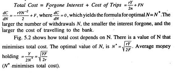
This expression shows that the individual holds money if the fixed cost of withdrawal F is higher, if expenditure Y is higher or if the interest rate r is lower.

So far, we have been interpreting the Baumol-Tobin model as a model of the demand for currency. But one can interpret the model more broadly. Suppose a person holds a portfolio of monetary assets and non-monetary assets.

Let r be the difference in the return between monetary and non-monetary assets, and let F be the cost of transferring non-monetary assets into monetary assets, such as brokerage fee. The decision about how often to pay a brokerage fee is analogous to the decision about how often to withdraw money from bank.

Thus, the Baumol-Tobin model describes this person’s demand for monetary assets. By showing that money demand depends positively on Y and negatively on r, the model provides a micro-economic justification for the money demand function, L (r, Y).

Model # 3. Keynesian Model of Income Determination:

In the simple closed economy model without government, the aggregate demand for output, derived from aggregate expenditure, has two parts — the consumption expenditure and the investment expenditure. We assume that the consumption expenditure is a linear function of income and investment expenditure is given autonomously.

The model is represented by the following two equations: (3) C = a + bY and (4) I̅= A, a positive constant. The consumption function is such that the marginal propensity to consume (mpc) is given by ∆C/∆Y = b, where b is a positive function lying between 0 and 1. The aggregate demand as a function of income is given by a + b(Y) + I̅.

Income attains the equilibrium value, when the following condition is satisfied:

(5) Y = a + b (Y) + I̅

Alternatively, we can derive the saving function from the consumption function and use the equation S = I as the condition for equilibrium. The model may be written as:

(6) S = S(Y) or, S = – a + (1 – b) Y

(7) I = a positive constant

(8) S(Y) =  I̅ or, – a + (1 – b) Y =  I̅

The saving function is derived from the consumption function in the following way:

S = Y – C = Y – (a + bY) .^.. S = – a + (1 – b) Y, where the marginal propensity to save: ∆S/∆Y = (1 – mpc) = (1 – b)

Solving either equation (5) or equation (8) for Y, we get the value of equilibrium income. For a graphic solution of equation (5) the consumption function is at first plotted in the graph and then the constant amount of investment expenditure is added to it to produce the aggregate demand curve. In Fig. 4.2, the a + bY is the consumption function and a + bY + I curve is the aggregate demand function. The a + bY + I curve is parallel to the consumption function, as the vertical distance between the two curves stands for the constant amount of the autonomously given investment expenditure.

Then, a  45° line is drawn from the origin as OE which gives the equality between income (Y) and the aggregate expenditure. The point of intersection between a + bY +  I̅ curve and the 45° line gives the solution of equilibrium for Y. Here Y_e is the equilibrium income. For a graphic solution of equation (8) the saving function is plotted on the graph, and then, the horizontal investment function is drawn. The intersection between the saving function and investment function gives the solution of equation (8) for Y. In the same figure (Fig. 4.2) this solution produces the same equilibrium income, Y_e.

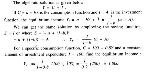
The same equilibrium income can be obtained from the saving function; when consumption function is C = 100 + 0.8Y, S = – 100 + (1 – 0.8) Y and I = 100,

S =  I̅ or, – 100 + 0.2Y = 100

.^.. Y_e =1/0.2 (100 + 100) = 1,000

The reason why income is settled at the equilibrium level is this: If income lies below Y_e, say at Y_A. aggregate expenditure (C + I) exceeds Y (or I exceeds S), implying that there is an excess demand for output, which leads to an increase in K; conversely, if income is above. Y_e, say at Y_B, aggregate expenditure (C + I) falls short of Y_e (or I is less than S), implying that there is excess supply which leads to a fall in Y. This shows that whenever income is not in equilibrium, it automatically moves towards equilibrium.

This movement also ensures the attainment of equilibrium, if it is a stable equilibrium. The stability condition requires that mpc in this model must be less than one. Thus, we can determine the equilibrium income with the help of a consumption function and an autonomously given investment function by solving the equation, Y = a + bY + I, for Y, only if mpc = ∆C/∆Y is less than 1. Herein lies the importance of the assumption that 0 < mpc < 1. Without this assumption the equilibrium condition becomes useless, as the equilibrating condition does not work. Thus mpc < 1, is the stability condition and where mpc = 1, multiplier is it is unstable condition.

The equilibrium condition discussed above has to be supplemented by the following adjustment hypothesis:

(9) dY /dt = λ (a + bY) + I – Y = λ [I – a + (1 – b)Y],

where λ is a positive adjustment factor.

The positive value of the dynamic adjustment coefficient λ can be justified in two ways. First, if prices are rigid, the excess demand (supply) will give signal to the producers to increase (decrease) production through (an increase) a decrease in inventories. Second, in a system of flexible prices, the signal will come from the increase (decrease) in prices in the presence of excess demand (supply).

The excess demand function can be linearised by taking the first two terms of Taylor’s series expansion around the equilibrium value, Y_e. Then equation (9) becomes a first order linear differential equation, the solution of which will give us the same dynamic stability condition, viz, mpc < 1, as we derived earlier with the help of the static analysis.

The simple Keynesian model has two parameters: the mpc and the autonomous investment function. A change in any one of the parameters will lead to a change in equilibrium income. An increase in the mpc will make both consumption function and aggregate expenditure function steeper in Fig. 4.2; and, then, equilibrium income will go up. An increase in autonomous investment expenditure will produce a parallel upward shift in the aggregate expenditure (aggregate demand) function in Fig, 4.2 which will also increase equilibrium income.

Model # 4. Complete Keynesian Model of Money Supply:

The complete Keynesian model can also be represented graphically by bringing together all the markets. We can identify from the diagram the equilibrium values of all the variables of the system. The Fig. 8.13 depicts the complete Keynesian model.

The figure shows the aggregate demand and aggregate supply (AS) curves. The aggregate demand curve is drawn on the assumption of a constant money supply M₀. The aggregate supply curve, AS, intersects the AD to produce equilibrium price level P̅ and the equilibrium output level Y̅, when the level of output is known, the corresponding level of employment N̅ can be obtained from the aggregate production function {r = f(N, K₀)}.

The labour demand and supply curves are drawn on the left hand side of the aggregate production function. The labour demand curve is drawn for the price level P̅. The labour demand curve intersects the labour supply curve to give us equilibrium employment N.

Since the labour demand curve intersects the labour supply curve at the latter’s horizontal part, there is involuntary unemployment of N_f – N̅. The equilibrium money wage rate is W₀. We have drawn the IS and LM curves above the AD and AS curves. The LM curve corresponds to the money supply M₀ and the equilibrium price level P. At the intersection of IS and LM curves the equilibrium rate of interest r is determined. From this diagram (Fig. 8.13), we can determine all important variables of the system.

Again, when Y is known, S can be determined from the saving function S(Y) which we have drawn above the IS-LM curves. When the equilibrium level of income is Y̅, the saving is S̅. The equality between saving and investment is shown through 45° line.

When the equilibrium rate of interest is known, the level of investment can be known from the diagram below the 45° line and to the left hand side of the IS-LM curves which give the equilibrium rate of interest. By extending the diagram, it is possible to show the transactions and the speculative demand for money separately which is avoided here.

In this way, all the equations of Keynesian model may be represented. The equilibrium system represented here is an underemployment equilibrium because there exists involuntary unemployment of N_f -N̅ which has been caused by wage rigidity. The full employment equilibrium may also be achieved if the labour demand curve intersects the supply curve at the latter’s upward rising part.

Some Special Criticisms of the Keynesian Model:

There are two general criticism of the Keynesian model. Firstly, the Keynesian model is “too aggregative”. Secondly, this model is too static. It means that the model does not consider the short-run dynamics of income change and that it is unsuitable to the analysis of long-term economic growth. The model is a short run model in that it assumes a given capital stock. Keynes was interested in the short run as he said, “in the long run we are all dead”.

The Keynesian model can be dynamised at least in two directions. Firstly, it is possible to introduce time lags in different functions and analysis of the time path to achieve different equilibrium values. Secondly, it may be possible to consider the effect of an increase in the capital stock on the equilibrium values of different variables. The model is “too static” for the analysis of either the problems of economic growth or the business cycle.

Apart from these general criticisms, we can advance some criticisms devoted to the specific parts of the Keynesian model.

Firstly, the Keynesian liquidity preference function has been criticised mainly on the ground that he considered only two assets — money and bonds. This is an over-simplification. In the real world, there are different types of monetary and non-monetary assets. All these are considered in the modern portfolio approach to the demand for money. Keynes’ division of the demand for money into three parts — transaction demand, precautionary demand and speculative demand — has also been criticised. It has been argued that it is difficult to separate between units of money held for speculative and transaction purposes. The same unit of money may be used for either purpose.

Secondly, the Keynesian investment theory has been criticised and new theories have been offered as an alternative to the Keynesian theory which have been discussed later in this book.

Thirdly, the Keynesian consumption function has been criticised and several alternative hypothesis has been developed which we consider later on.

Fourthly, the hypothesis that firms maximise profits has been criticised. Recent developments of the theory of firms show that the objective of the modern firms is not only the maximisation of profits. There are alternative objectives such as sales revenue maximisation and managerial utility maximisation and so on.

Model # 5. The Mundell-Fleming Model:

The Mundell-Fleming Model is made up of the following three equations:

IS: C(Y – T) + I(r) + G + NX (e)

LM: M/P = L(r, Y)

r = r*

We review each of these equations before putting them together to make a short-run model of a small open economy. The first equation describes the goods market. It is already familiar to us—the aggregate Y is the sum of consumption C, investment I, government expenditure G, and net exports NX. Consumption depends on disposable income (Y -T). Investment is negatively related to interest rate(r). Net exports depend negatively on the real exchange rate(e).

Since the Mundell-Fleming Model assumes that prices are fixed, changes in the real exchange rate are proportional to changes in the nominal exchange rate and when the nominal exchange rate rises, foreign goods become less expensive compared to domestic goods—which stimulates imports and depresses exports. The second equation is a familiar money market equation, which states that the supply of real money balances, M/P, equals the demand, L(r, Y).

The demand for money depends negatively on the interest rate and positively on income. The money supply is an exogenous variable controlled by the monetary authority. Like the IS-LM Model, the Mundell-Fleming Model takes the price level P as an exogenous variable.

The third equation states that the world interest rate r* determines the interest rate in the economy. This equation holds because we are examining a small open economy which is sufficiently small relative to the world economy wherefrom it can borrow or lend as much as it wishes without affecting the world interest rate. These three equations fully describe the Mundell-Fleming Model. We will examine the implications of these equations for short-run fluctuations in an open economy.

Model # 6. Bent Hansen’s Model of Demand-Pull Inflation:

Hansen’s Model of demand inflation shows that the simultaneous increase in the money wage rate and the price level are the products of the inflationary gaps in both the labour market and the output market. When the aggregate demand for labour exceeds its full employment supply, the inflationary gap appears in the labour market, and when the aggregate demand for output exceeds its full employment supply, the inflationary gap appears in the output market.

When the inflationary gap appears in the output market, consequence is a rise in the price level, and when it appears in the labour market, the result is a rise in the money wage rate. The wage rate will increase only if there is excess demand for labour.

Even if there is no excess demand for output the price level can go up due to an increase in the wage rate. Hansen points out that, in an inflationary process, there is an interaction between the two markets; inflationary gaps appear in both markets and both prices and money wages rise simultaneously.

The existence of inflationary gap in the output market ensures its existence in the labor market, and vice versa. As a con­sequence, both the money wage rate and the price level rise in such a way as to keep the real wage rate, the real output and the size of the inflationary gaps constant.

If the full employment supply of output is autonomously given, the in­flationary gap in the output market can be expressed as the difference between the actual demand and the full employment supply. The inflationary gap in the labour market may be expressed in two ways: the difference between the actual demand for labour and its full employment supply, and the difference between the intended and the actual supply of output.

The intended supply of output generates the demand for labour, and it is the second difference which gives a measure of the inflationary gap in the market in terms of the unfulfilled supply plans of the producers. In this analysis, we shall use the second expression of the inflationary gap in the labour market, which enables us to express both the inflationary gap in the same unit.

The aggregate demand for output (AD) may be expressed as an increasing function of the real wage rate (W/P). If wage income rises with the rise in the real wage rate and if the marginal propensity to spend of the workers is greater than that of the profit-earners, we can assume that, an increase in the real wage rate will lead to an increase in the aggregate demand for output. The intended supply of output (AS) may be assumed to be a decreasing function of the real wage rate.

The diminishing marginal productivity of labour and the principle profit-maximisation explain why a rise in the real wage rate leads to a fall in the intended supply of output. It is assumed that the full employment output (S_f) is independent of the real wage rate. The inflationary gap in the output market is defined as (AD – S_f), and the rate of increase in the price level over time is assumed to be a monotonically rising function of the inflationary gap in the output market.

Thus, the following functional relation can be written as, dp/dt = f (AD – S_F), where dp/dt = 0 for f(0) and the first derivative of the function f’ > 0. The inflationary gap in the labour market is defined as AS – S_f, and the rate of increase in the money wage (W_m) rate over time is assumed to be a monotonically rising function of the inflationary gap in the labour market. Thus, we have the following functional relationship: dw/dt = F (AS – S_f), where dw/dt = 0 for F (0) and its first derivative F’ > 0.

These assumptions of the last paragraph will generate a model of demand inflation in which the simultaneous rises in the money wage rate and the price level can be explained. Diagrammatic presentation of the model is presented in Fig. 16.10. In part 16.10(a), the positively sloped AD curve and the vertical line is the full employment supply curve. When the full employment supply curve passes through the point of intersection between the AD curve and the intended supply curve, there is equilibrium in both markets.

Given the full employment supply curve, the point of intersection between the AD curve and the AS curve may shift to the right of the S_f line, when conditions of disequilibrium are created in both markets. The rightward shift of the point of intersection is brought about by autonomously produced rightward shifts in the AD – curve and the AS – curve.

These autonomous shifts are the inflation- producing factors that are mainly responsible for the conditions of disequilibrium in the economy. Once the point of intersection between the AD-curve and the AS-curve goes to the right of the S_f -curve, inflationary gap arise in both markets.

At the real wage rate W’/P’ there is no inflationary gap in the labour market, though there is an inflationary gap in the product market. As a result, the price level rises and the real wage rate falls. Thus, at W’/P’, the real wage rate is the highest and it is bound to fall. With the fall in the real wage rate below W’/P’, an inflationary gap also appears in the labour market.

The simultaneous existence of inflationary gaps in both markets leads to rises in prices and wages. Again, at the lowest real wage rate of W”/P”, there is an inflationary gap in the labour market, though no such gap exists in the product market. But, the money wage rate rises leading to a rise in the real wage rate.

As a result, inflationary gaps arise in both markets and both P and wage increase. Thus, it follows that the real wage rate must be between these two limits, where it will exactly lie depends on the two functions dp/dt = f (RD – S_f) and dw/dt = F(AS – S_f). If dp/dt = dw/dt, both markets are in equilibrium.

If they are not equal [dp/dt ≠ dw/dt], the real wage rate changes, leading to changes in the respective inflationary gaps in the two markets. As a result, dp/dt rises and dw/dt falls. Thus, dp/dt and dw/dt always move forwards equality. If dp/dt < dw/dt, the real wage rate rises, and then the inflationary gap in the output market rises and that in the labour market falls. If, on the other hand, dp/dt > dw/dt, the real wage rate falls and the inflationary gap in the output market falls and that in the labour market rises. Thus, dp/dt falls and dw/dt rises.

This can be seen in Fig. 16.10(b) where the two functions, dp/dt and dw/dt, are presented and shown on the f-curve and F-curves, respectively. The origin of the figure in 16.10(b) has been placed at a particular point, so that the respective inflationary gaps in it equal to those in 16.10(a).

The positions of the two functions in 16.10(b) depends on their sensitivities to the respective inflationary gaps. If dp/dt is more sensitive to (AD – S_f) than dw/dt to (AS – S_f), the f-curve will lie to the left of the F-curve, meaning that the inflationary gap in the output market will be less than that in the labour market to make dp/dt = dw/dt.

If, however, the f-curve lies to the right of the F-curve, then dp/dt = dw/dt would be at a greater inflationary gap in the output market than that in the labour market. In Fig. 16.10(b) the curves have been drawn under the assumption that dp/dt is less sensitive to the inflationary gap in the output market than dw/dt to that in the labour market. During the inflation, a position of quasi-equilibrium is reached, when dp/dt = dw/dt.

Then, w/p becomes constant and the inflationary gaps remain unchanged, leading to rises in the price level and the money wage rate at a constant rate. In the Fig. 16.10(b) W/P is constant real wage rate which prevails in quasi-equilibrium position. O’L is the rate of increase in P and W. If the f-curve lies to the right of the f-curve, the position of w_e/p_e will be located above the point of intersection between the AD-curve and the AS- curve.

In the opposite case, it will lie below that point. When dp/dt and dw/ dt are equally sensitive to the respective inflationary gaps, the two curves in Fig. 16.10(b) will coincide with each other and W_e/P_e will lie at the point of intersection between the AD-curve and the AS-curve.

Model # 7. The Kaldor-Mirrlees Model:

Kaldor has developed two models of economic growth (1957, 1962). Here we shall briefly concentrate with the one developed by Kaldor and Mirrlees (KM) in 1962. The crucial feature of this model is that the saving ratio can be made flexible to obtain a steady-state economic growth. Unlike the neo­classical model, the capital-output ratio remains fixed.

Note that the KM model discards the production function approach of the neo-classical theory and introduces a technical progress function. The neo-classical school has not specified any investment function; but, in the KM model, an investment function is specified which depends upon a fixed pay-off period for investment per worker.

The assumptions regarding both full-employment and perfect com­petition are dropped.

Instead, K and M start off with the assumption that total income Y is equal to the sum of wages W and profits P:

Y = W + P………. (1)

Total savings S = S_w + S_p…… (2)

Note that, S = S_wW + S_pP…… (3)

and S_w = S_wW……. (4) S_p= S_pP………. (5)

where S_w is the propensity to save by wage earners, S_p is the propensity to save by profit earners and S is total savings. Both S_w and S_p are assumed to be constant indicating the equal i ty between marginal and average propensities.

Now Y = W + P and 5 = S_w W + S_pP

By substitution, we have S = S_w(Y – P) + S_pP…….. (6)

S = (S_p– S_w) + S_WY……… (7)

Since it is assumed that I = S…………….. (8)

we have I = (S_p – S_w) P + S_WY…………. (9)

Dividing both sides of the equation by Y and rearranging we obtain:

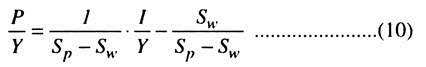
Thus, the profit share of income is given by the share of investment to income. The stability of the model is given by 0 < S_w < S_p <1. Notice that the flexibility of saving is achieved in the KM model by the assumption of different propensities to save by wage and profit earners.

The specific value of savings necessary to obtain the solution would be given by income distribution between income classes. Given S_p and S_w, l/Y will determine P/Y. If it is assumed that S_w = 0, we then obtain – P/Y = 1/S_w x 1/Y ……… (11)

Note that, if the capital-output ratio K/Y is fixed as in the HD model, we can write:

Since P/K = Y, the rate of profit .earned on capital, and I/K = J, the rate of accumulation, we have v = 1/S_p j or, S_pv = J……… (13).

This conclusion betrays remarkable affinity to the Von Neumann case, where Neumann puts S_p = 1. Thus, all profits are saved and in equilibrium we obtain V = J(=n) where n is the natural growth rate, which is assumed thus: the rate of growth is given by the rate of profit which is determined by the propensity to save of the profit earners.

Kaldor’s introduction of an ‘alternative’ theory of distribution to analyse the problem of economic growth is interesting. However, several important criticisms have been leveled at the Kaldor’s theory.

First, Pasinethi mentions a ‘logical slip’ in Kaldor’s argument when he observed that, although he has allowed workers to save, he did not allow these savings to accumulate and generate economic growth. Pasinethi has demonstrated that on a steady-state growth path the profit rate depends only on the growth rate and the propensity to save by the capitalists, it is independent of the propensity to save by the workers.

However, if it is assumed that capitalists as a class have been banished and capital is owned by the workers alone, than the relevant variables in the balanced growth path will be given by S_w and n. Second, Kaldor’s assumption about the fixed propensities to save disregards the impact of life cycle on save and work. Third, the assumption of a fixed class of income receivers is regarded as unrealistic.

Finally, Kaldor’s Model fails to exhibit an explicit behavioural mechanism, which will ensure that the actual distribution of income will be such as to maintain the steady-state growth path.

 

Model # 8. Solow’s Model of Growth:

Prof. Robert M. Solow made his model an alternative to Harrod-Domar model of growth. It ensures steady growth in the long run period without any pitfalls. Prof. Solow assumed that Harrod-Domar’s model was based on some unrealistic assumptions like fixed factor proportions, constant capital output ratio etc.

Solow has dropped these assumptions while formulating its model of long-run growth. Prof. Solow shows that by the introduction of the factors influencing economic growth, Harrod-Domar’s Model can be rationalised and instability can be reduced to some extent. He has shown that if technical coefficients of production are assumed to be variable, the capital labour ratio may adjust itself to equilibrium ratio in course of time.

In Harrod-Domar’s model of steady growth, the economic system attains a knife-edge balance of equilibrium in growth in the long-run period. This balance is established as a result of pulls and counter pulls exerted by natural growth rate (Gn) (which depends on the increase in labour force in the absence of technical changes) and warranted growth rate (Gw) (which depends on the saving and investment habits of household and firms).

However, the key parameter of Solow’s model is the substitutability between capital and labour. Prof. Solow demonstrates in his model that, “this fundamental opposition of warranted and natural rates turns out in the end to flow from the crucial assumption that production takes place under conditions of fixed proportions.” The knife edge balance established under Harrodian steady growth path can be destroyed by a slight change in key parameters.

Prof. Solow retains the assumptions of constant rate of reproduction and constant saving ratio etc.” and shows that substitutability between capital and labour can bring equality between warranted growth rate (Gw) and natural growth rate (Gn) and economy moves on the equilibrium path of growth.

In other words, according to Prof. Solow, the delicate balance between Gw and Gn depends upon the crucial assumption of fixed proportions in production. The knife edge equilibrium between Gw and Gn will disappear if this assumption is removed. Solow has provided solution to twin problems of disequilibrium between Gw and Gn and the instability of capitalist system.

In short, Prof. Solow has tried to build a model of economic growth by removing the basic assumptions of fixed proportions of the Harrod-Domar model. By removing this assumption, according to Prof. Solow, Harrodian path of steady growth can be freed from instability. In this way, this model admits the possibility of factor substitution.

Assumptions:

Solow’s model of long run growth is based on the following assumptions:

1. The production takes place according to the linear homogeneous production function of first degree of the form

Y = F (K, L)

Y — Output

K — Capital Stock

L — Supply of labour force

The above function is neo-classic in nature. There is constant returns to scale based on capital and labour substitutability and diminishing marginal productivities. The constant returns to scale means if all inputs are changed proportionately, the output will also change proportionately. The production function can be given as aY = F (aK, al)

2. The relationship between the behaviour of savings and investment in relation to changes in output. It implies that saving is the constant fraction of the level of output. In this way, Solow adopts the Harrodian assumption that investment is in direct and rigid proportion to income.

In symbolic terms, it can be expressed as follows:

I = dk/ dt = sY

Where

S—Propensity to save.

K—Capital Stock, so that investment I is equal

3. The growth rate of labour force is exogenously determined. It grows at an exponential rate given by

L = L₀ e^nt

Where L—’Total available supply of labour.

n—Constant relative rate at which labour force grows.

4. There is full employment in the economy.

5. The two factors of production are capital and labour and they are paid according to their physical productivities.

6. Labour and capital are substitutable for each other.

7. Investment is not of depreciation and replacement charges.

8. Technical progress does not influence the productivity and efficiency of labour.

9. There is flexible system of price-wage interest.

10. Available capital stock is fully utilized.

Following these above assumptions, Prof. Solow tries to show that with variable technical co-efficient, capital labour ratio will tend to adjust itself through time towards the direction of equilibrium ratio. If the initial ratio of capital labour ratio is more, capital and output will grow more slowly than labour force and vice-versa.

To achieve sustained growth, it is necessary that the investment should increase at such a rate that capital and labour grow proportionately i.e. capital labour ratio is maintained.

Solow’s model of long-run growth can be explained in two ways:

A. Non-Mathematical Explanation.

B. Mathematical Explanation.

 

A. Non-Mathematical Explanation:

According to Prof. Solow, for attaining long run growth, let us assume that capital and labour both increase but capital increases at a faster rate than labour so that the capital labour ratio is high. As the capital labour ratio increases, the output per worker declines and as a result national income falls.

The savings of the community decline and in turn investment and capital also decrease. The process of decline continues till the growth of capital becomes equal to the growth rate of labour. Consequently, capital labour ratio and capital output ratio remain constant and this ratio is popularly known as “Equilibrium Ratio”.

Prof. Solow has assumed technical coefficients of production to be variable, so that the capital labour ratio may adjust itself to equilibrium ratio. If the capital labour ratio is larger than equilibrium ratio, than that of the growth of capital and output capital would be lesser than labour force. At some time, the two ratios would be equal to each other.

In other words, this is the steady growth, according to Prof. Solow as there is the steady growth there is a tendency to the equilibrium path. It must be noted here that the capital-labour ratio may be either higher or lower.

Like other economies, Prof. Solow also considers that the most important feature of an underdeveloped economy is dual economy. This economy consists of two sectors-capital sector or industrial sector and labour sector or agricultural sector. In industrial sector, the rate of accumulation of capital is more than rate of absorption of labour.

With the help of variable technical coefficients many employment opportunities can be created. In agricultural sector, real wages and productivity per worker is low. To achieve sustained growth, the capital labour ratio must be high and underdeveloped economies must follow Prof. Solow to attain the steady growth.

This model also exhibits the possibility of multiple equilibrium positions. The position of unstable equilibrium will arise when the rate of growth is not equal to the capital labour ratio. There are other two stable equilibrium points with high capital labour ratio and the other with low capital labour ratio.

If the growth process starts with high capital labour ratio, then the development variables will move in forward direction with faster speed and the entire system will grow with high rate of growth. On the other hand, if the growth process starts with low capital labour ratio then the development variables will move in forward direction with lesser speed.

To conclude the discussion, it is said that high capital labour ratio or capital intension is very beneficial for the development and growth of capitalist sector and on the contrary, low capital-labour ratio or labour-intensive technique is beneficial for the growth of labour sector.

B. Mathematical Explanation:

This model assumes the production of a single composite commodity in the economy. Its rate of production is Y (t) which represents the real income of the community. A part of the output is consumed and the rest is saved and invested somewhere. The proportion of output saved is denoted by s. Therefore, the rate of saving would be sY (t). The capital stock of the community is denoted by K it). The rate of increase in capital stock is given by dk/dt and it gives net investment.

Since investment is equal to saving so we have following identity:

K = sY … (1)

Since output is produced by capital and labour, so the production function is given by

Y = F (K, L) … (2)

Putting the value of Y from (2) in (1) we get

S = s F (K, L) … (3)

Where

L is total employment

F is functional relationship

Equation (3) represents the supply side of the system. Now we are to include demand side too. As a result of exogenous population growth, the labour force is assumed to grow at a constant rate relative to n. Thus,

L (t) = L₀e^nt …(4)

Where

L—Available supply of labour

Putting the value of L in equation (3) we get

K = sF (K, L₀e^nt) …(5)

The right hand of the equation (4) shows the rate of growth of labour force from period o to t or it can be regarded as supply curve for labour. “It says that the exponentially growing labour force is offered for employment completely in elastically. The labour supply curve is a vertical line, which shifts to the right in time as the labour force grows. Then the real wage rate adjusts so that all available labour is employed and the marginal productivity equation determines the wage rate which will actually rule.”

If the time path of capital stock and of labour force is known, the corresponding time path of real output can be computed from the production function. Thus, the time path of real wage rate is calculated by marginal productivity equation.

The process of growth has been explained by Prof. Solow as, “At any moment of time the available labour supply is given by (4) and available stock of capital is also a datum. Since the real return to factors will adjust to bring about full employment of labour and capital we can use the production function (2) to find the current rate of output. Then the propensity to save tells us how much net output will be saved and invested. Hence, we know the net accumulation of capital during the current period. Added to the already accumulated stock this gives us the capital available for the next period and the whole process can be repeated.”

Model # 9. Meade’s Model of Economic Growth:

Prof. J.E. Meade in his book ‘A Neo-classical Theory of Economic Growth’ constructed model to study the process of equilibrium growth i.e. steady-state growth. In fact, the model is designed to show the way in which the simplest form of classical economic system would behave during a process of equilibrium growth.

This model provides the relation to increase the income and population. It analyses the influence of income, capital, labour and technology on development. It also gives the conditions under which the growth of economy is possible. He tries to establish a relationship between population growth and income growth.

Meade states three principles on which the economy grows. They are the following:

1. Capital accumulation resulting from the savings made out of current income.

2. Growth of working population i.e. growth of labour force.

3. Technical progress which allows more and more output to be produced by a given amount of resources.

Prof. Meade in his model examined the behaviour of competitive economy during the process of equilibrium growth when real capital is being accumulated, labour force is growing and technical progress is accruing. Therefore he tries to incorporate these variable factors in classical model and to find out how the economy behaves under these conditions.

 

Assumptions:

In constructing his growth mode, Prof. Meade assumes following assumptions:

1. The economy is classed as having no economic or financial relations with other countries.

2. The production in the economy is assumed to take place under the conditions of perfect competition.

3. Complete Laissez-faire is assumed to prevail in the economy i.e. the economy is working under the conditions of constant returns to scale.

4. The economy is producing in two types of commodities- consumption goods and capital goods. The consumption goods satisfy all the human needs of consumption and the capital goods are used to produce capital goods.

5. Machines are the only form in which the capital is assumed.

6. The factors of production, land and labour are assumed to be in a state of full employment.

7. The money price of consumption goods is considered to be constant.

8. There are no State or Governmental economic activities involving taxation or state expenditure.

9. The production function can be substituted for one another. In a state of technical knowledge, it is possible to produce the consumption goods or capital goods by a more labour intensive method or a more land intensive method or by a more machinery intensive method, depending upon the availability of cheap labour.

10. The machines and labour are substituted for each other. It has been assumed that all machines are alike and can be altered in any desired way, both in short run and long run.

11. It is also assumed that at every moment of time, the production function for a unit of consumption good is the same as the production function for a unit of capital good. This assumption is called Perfect Substitution in production between capital goods and consumption goods.

12. Each year, a certain percentage of machinery depreciates and needs replacement. This is called assumption of depreciation by evaporation.

Model # 10. Joan Robinson’s Model of Growth:

Mrs. Joan Robinson has given her model of growth in her classic book. ‘The Accumulation of Capital’ in 1956. Joan Robinson’s model clearly takes the problem of population growth in a developing economy and analyses the influence of population on the role of capital accumulation and growth of output. In words of Prof. Mathew, The relation between distribution and growth in this model arises partly from the mutual interdependence of the rate of profit and the pace of capital accumulation and partly from the effect of distribution of income on the proportion of income saved.

The two fundamental propositions of the model are as under:

1. The capital formation depends on the manner of distribution of income.

2. The rate at which labour is utilized depends upon the supply of capital and that of labour.

Assumptions:

1. Labour and capital are the only productive factors. It implies that the national output is the result of combined efforts of these two factors of production.

2. The economy is assumed to be closed i.e. there is no foreign trade.

3. Total wage bill is the product of real wage rate and number of workers.

4. Total income is divided between capital and labour as these are the two factors of production.

5. The production is not affected by the technological changes i.e. there is no progress in technology.

6. Total profit is the product of profit rate and amount of capital invested.

7. There is constancy in price level.

8. Wage earners spend all of their wage income on consumption, while profit takers save and invest all of their profit income.

9. Capital and labour are combined in a fixed proportion for a given output.

10. The national income is the sum of wage bill and total profits.

11. There is no scarcity of labour and entrepreneurs can employ as much labour as they wish.

12. Entrepreneurs consume nothing but save and invest their entire income for capital formation. If they have no profits, there is no accumulation and if they do not accumulate, they have no profits.

Open Model:

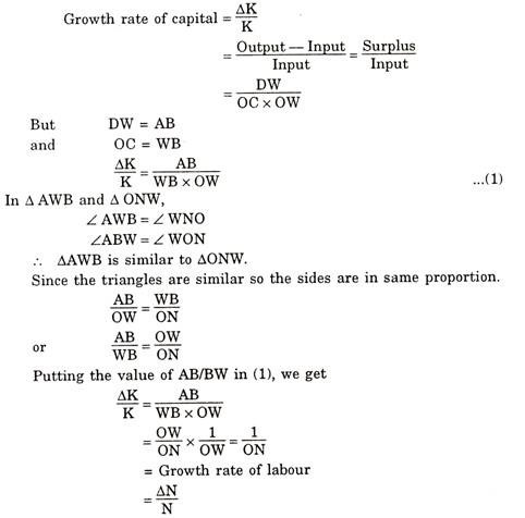
In an open economy, the conditions for the steady growth and conditions for rising rate of capital accumulation will be discussed. According to Mrs. Joan Robinson, national income is the sum of the total wage bill and total profit. Total wage bill is the real wage multiplied by the number of workers and total profits are equal to profit rate multiplied by the amount of capital.

This relationship can be expressed as under:

PY = WN + πPK

Where P — Average Price level.

Y— Net national income.

W — Net money wage rate.

N— Amount of labour employed.

K— Amount of capital invested.

π — Rate of profit.

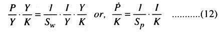
To convert the expression into real terms, divide both sides of equation by p (average price level), we get:

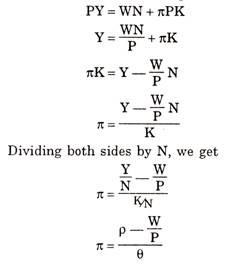
Where ρ Y/N i. e Labour/ Productivity, W/P real wage rate

θ = K/N i.e., Capital Labour Ratio

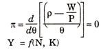
The above equation indicates that the profit rate is a function of labour productivity (p) and real wage rate (W/P) and capital labour ratio (8). In other words, the profit rate is shown as capable of varying directly with the rate of net return to capital and inversely with the coefficient of capital intensity. The necessary condition for maximization is that the first derivative must be zero.

Keynesian income expenditure analysis shows that the net national real income (Y) is the sum of real consumption expenditure (C) and real net investment which can be expressed as:

Y = C + I

Now we know that labour spends its entire income and saves nothing. The profit earning class makes saving in the form of profit. According to Mrs. Robinson, savings must be equal to total profits. Thus, savings in a given period are equal to capital investment multiplied by rate of profit.

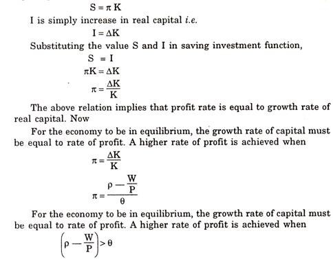
The above equation illustrates that the rate of growth of capital is capable of increasing if the net returns to capital rise in greater proportion than the capital-labour ratio and vice-versa. In other words, lower rate of profit always affects the supply of capital adversely which in turn widens the gap between supply of capital and labour. The main feature of the model is that the rate of growth of capital is dependent on profit rate.

Closed Model:

In a closed economy, the concepts of Golden age and Platinum age are to be discussed. In simple words, Golden age is a situation of smooth steady growth with full employment arising out of the equality of the ‘Desired’ and ‘Possible’ rates of accumulation and has been designated by Mrs. Joan Robinson as the Golden age equilibrium. However, if an increase in labour supply is not accompanied by proportionate increase in the capital supply, then it will cause unemployment in the economy. To achieve full employment of labour the growth rate of population must be equal to growth rate of capital i.e.

∆N/N = ∆K/K

When the rate of growth of labour and capital are equal to each other, then there is full utilisation of capital in the economy. Such a switch on is called Golden age. The existence of Golden age is the indicator of full employment level.

The concept of Golden age implies that there must be equality in actual, warranted and natural growth rates. In short, in Mrs. Robinson Joan’s words, when technical progress is neutral and proceeding steady, without any change in the time pattern of production, the competitive mechanism works freely, population grows (if at all) at a steady rate and accumulation goes on fast enough to supply productive capacity for all available labour, the rate of profit tends to be constant and the level of real wages rises with output per head. Then there are no internal contradictions in the system, we may describe these conditions as a Golden age (thus indicating that it represents a mythical state of affairs not likely to obtain in any actual economy). This is explained with the help of a diagram 1.

In the figure 1, capital labour ratio is illustrated along positive direction of X-axis and wage rate of labour on Y-axis and the growth rate of labour on negative side of X-axis. The production function is represented by OP. Each point on this curve shows the proportion in which capital and labour are combined to produce a particular level of output.

Tangent NT touches the curve OP at A and intersects Y-axis at W. At point A capital labour ratio is OC, the productivity of labour is OD and out of which OW is the wage rate. The surplus DW is rate of return to capital. The point A shows the position of equilibrium because the slope of tangent NT and the slope of production curve OP is the same. It can also be said that at A, the growth rate of capital ∆K/K is equal to growth rate of labour ∆N/N.