Concepts of Cost: Top 8 Concepts | Capital

The following points highlight the eight main concepts of cost. The concepts are: 1. Cost of Loan Capital 2. Cost of Equity Capital 3. Risk-Free Rate Plus Risk Premium 4. Dividend Capitalisation Approach 5. Capital Asset Pricing Model (CAPM) 6. Cost of Preference Shares 7. Cost of Retained Earnings (or Internal Equity) 8. The Composite or Overall Cost of Capital.

Concept # 1. Cost of Loan Capital:

The firm obtains loan capital by selling debentures. Generally, the nominal value and the net value of the debentures are not the same. This is because the firm may sell its debentures at par; it may sell the debentures also at a premium or at a discount.

In order to sell the debentures, the firm has to bear certain expenses, e.g., advertisement cost, brokerage and underwriting com­missions, etc. Therefore, we shall get the net value of the debentures if we subtract their selling expenses from the proceeds obtained from selling them.

Let us suppose that the firm has sold some debentures with a term of n years. Let us suppose that the nominal value of each debenture is P (Rs) and the net value is D_P (Rs). Now, if the rate of interest is r (0 < r < 1), and if the income tax rate is x (0 < τ < 1), then, since the money paid as interest is exempted from the estimates of income tax, the net r of the firm, in this case, would be

r_N = r(1 – τ)                          (20.1)

Therefore, for every year, up to the nth year, the firm would have to pay for every debenture an interest equal to Pr_N, or, Pr(1 – τ), and, in the nth year, along with interest, the principal amount to be repaid for every debenture would be P.

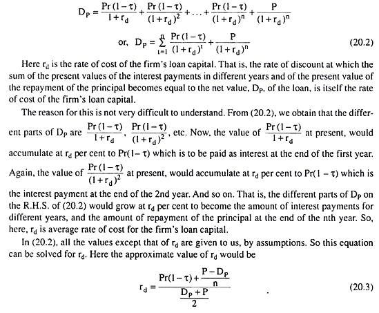
Let us now suppose that, at the rate of discount, r_d, we obtain:

 

 

 

 

 

 

 

 

 

 

 

 

 

 

 

 

 

Let us remember that if the debenture is a perpetuity (i.e., n = ∞), then equations (20.2) and (20.3) would give us:

Concept # 2. Cost of Equity Capital:

Generally, the supply of equity capital comes from the shareholders. People buy ordinary shares because they expect to obtain dividend from the company. If the shareholders actually obtain dividend at a rate which is lower than their expected rate, then the price of the share would be falling in the market.

On the other hand, if they obtain a rate higher than their expected rate then the market price of the share would be rising. The firm would have to invest the equity capital in such a way and it would have to earn profit at such high a rate that it would be able to pay dividend to the shareholders at least at their minimum expected rate. Then there would be no harm to the market price of the share.

The rate of dividend of ordinary shares is not fixed by contract. This rate would depend on the rate of profit acquired by the firm. The holder of ordinary shares may obtain dividend at a higher rate or at a lower rate or, some year, he may not obtain any dividend whatsoever.

That is why it may apparently seem that the equity capital has no cost. But this idea is not correct. The equity capital also has cost. However, since the dividend to be paid to the shareholders is not fixed beforehand, the process of estimating this cost is more complicated. In fact, from the investment of equity capital, the firm would have to earn profit at such a high rate that the shareholders may be paid a dividend at their minimum expected rate and the share price may be kept intact.

The minimum rate of dividend that the shareholders expect (r_e) is considered to be the cost of the equity capital. We shall now discuss some procedures of esti­mating this cost. We have to remember here that undistributed profit is not exempted from income tax. Therefore, income tax has no direct role to play in the determination of the cost of equity capital.

Concept # 3. Risk-Free Rate Plus Risk Premium:

Ordinarily, an investment in common stock is considered to be more risky than an investment in bonds. The firm is committed by contract to pay the interest and the principal sum to the bondholder—this money would have to be paid before the dividend is distributed among the shareholders. The rate of dividend, on the other hand, increases or diminishes according as the profit of the firm increases or diminishes.

But, barring exceptional economic crises, the firm is bound to pay the bondholder his dues at the predetermined rate. That is why it is thought that the rate of return (r_e) expected by the investor in equity capital should be equal to the sum of the risk-free return (r_f) of the bond (r_f is generally thought to be the risk-free return of the long-term government bonds) and a premium for bearing the risk.

In the case of investment in shares the risk may emerge from two sources. First, the risk for investing in the bonds of a private company instead of investing in government bonds. Second, some additional risk for investing in shares instead of investing in the bonds of the (private) company. We shall denote the premium associated with these two types of risk by e₁ and e₂, respectively.

Therefore, the cost rate of equity capital would be obtained to be:

r_e = r_f + e₁ + e₂                         (20.5)

or, r_e = r_f + e                              (20.5a)

where e = e₁ + e₂ = total rate of risk-bearing premium for investment in the common stock of a private company.

An easy way to have a measure of the first type of risk is to accept the difference between the rate of return on the bonds or debentures of the firm (r_d) and the rate of interest on govern­ment bonds (r_f) as e₁.

We therefore obtain:

e₁ = r_d – r_f                               (20.6)

The greater the risk associated with the private bonds, the greater would be the value of r_d and, consequently, the greater would be e₁.

On the other hand, a rule of thumb is used to obtain a measure of e₂. Here e₂ is not obtained on the basis of any formula or equation, it is obtained only on the basis of judgement. In this case, the financial analysts use a particular method.

They think that the return on the common stock of the firm (r_m) should be greater than the return on its bonds (r_d) by 3 per cent to 5 per cent.

If we accept the average of 3 per cent and 5 per cent, viz., 4 per cent, as the estimate of e₂, then the total rate of risk-bearing premium for investment in the common stock of a private company would be:

e = e₁ + e₂ [here it has been assumed that e₂ = r_m – r_d = 0.04]                      (20.7)

or, e = (r_d – r_f) + 0.04

For example, if the risk-free rate (r_f) is 10 per cent and the rate on the firm’s bonds (r_d) is 12 per cent, then the total rate of risk-bearing premium would be:

e = (0.12 -0.10) + 0.04 = 0.06

Therefore, in this case, firm’s cost of equity capital would be r_e = r_f + e = OTO + 0.06 = 0.16 or 16%.

We have to remember here that e is the difference between the risk on common stock and that on government bonds

e = e₁ + e₂ = (r_d – r_f) + (r_m – r_d) = r_m – r_f                                         (20.8)

Concept # 4. Dividend Capitalisation Approach:

The method of obtaining the estimate of cost of equity capital that we have discussed above, has considered the risks involved in the investment in equity capital but the fact that the rate of dividend and/or the price of the shares might also rise along with the passage of time has not been taken into account in that method.

We shall now discuss a method that would consider these points. This method is known as Dividend Capitalisation Approach (DCA).

The value of a firm is the sum total of the present values of all the profits that it expects to earn in future. In just the same way, the value of a share in the common stock is the sum-total of the present values of all the dividends that is expected to be obtained at different times in future.

The rate of discount at which these present values are obtained, would be taken to be the investor’s expected rate of return (r_e) from the share.

We obtain, therefore:

Here P₀ is the present market price of the common share and D₁, D₂, D₃,… are the dividend amounts obtained at the end of different years. Again, if it is thought that the dividend would be the same every year, then the flow of dividends from the share may be considered to be an annuity.

In this case, the value of the share would be equal to the present value of the said annuity.

If the expected annual dividend of each share is D₁ = constant, then the price or the value of the share would be:

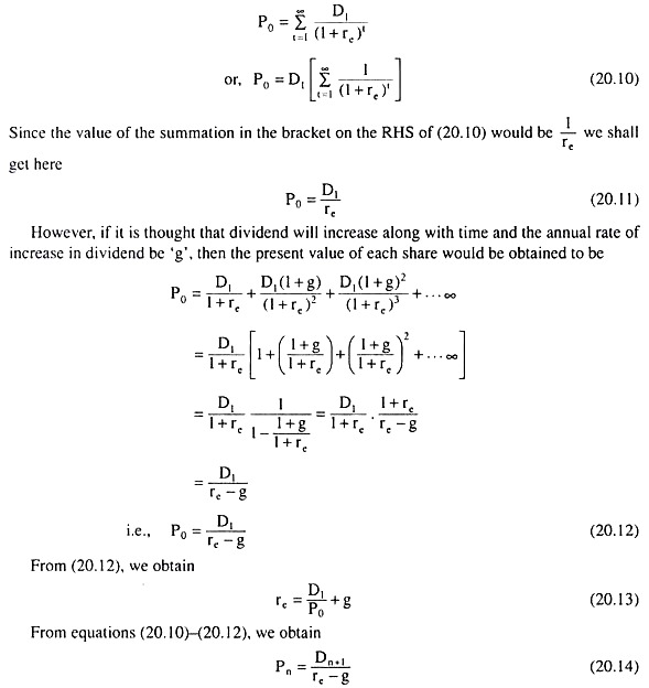
Here P_n is the expected price of the share at the end of the nth year and D_n+1 is the expected dividend at the end of the (n + 1)th year. Equations (20.9)-(20.15) are the relations between P and r_e. If we know the value of one of them, then the value of the other can be obtained from these equations.

We have to remember here that, while finding out the expected rate of return (r_e) from the price of the share, we should accept the net proceeds obtained from the sale of the share as its price. Let us suppose that a share of nominal value of Rs 100 is sold at a premium of 10 per cent and the selling expenses are 5% of the proceeds obtained.

Here the market price of the share will be P₀ = Rs 110 and the net proceeds from the sale of the share will be Rs 110 (1 – .05) or Rs P₀ (1 – h).

In this case, equation (20.13) will have to be duly modified and we would get:

Here h = proportion of selling expenses of a share in its market price (0 < h < 1). That is, the rate of return that the investors would expect from investing in equity capital, or, the cost of equity capital, would be the current dividend yield from the common stock (D₀/P) plus the expected rate of increase in dividend payments (g).

The historic rate of dividend growth of the firm or the unanimous rate of the financial analysts may be accepted as the estimate of g.

For example, let us suppose that the firm pays a dividend of Rs 6 for each share of the common stock and the financial analysts are unanimous that the annual rate of dividend growth would be 4 per cent.

Here, according to the Dividend Capitalisation Approach (DCA), the cost of equity capital of the firm would be:

r_e= 6/100 + 0.04

= 0.06 + 0.04 = 0.10, or, 10%.

Concept # 5. Capital Asset Pricing Model (CAPM):

We shall now discuss the Capital Asset Pricing Model (CAPM) of cost estimation of equity capital. While estimating the cost of equity capital of a particular company, this model consid­ers not only the difference between risk of its common stock and that of government bonds, but also the difference in risk that might exist between the stocks of different companies.

If we denote the average rate of return of the common stocks of different companies by r_m and the fixed rate of return of the government bonds by r_f, then the difference in risk between common stocks and government bonds would be r_m – r_f.

Let us now assume that, in a particular period of time, say, in one year, the return obtained from a share of common stock is the sum total of the dividend and the change in the share price obtained during the period.

Let us suppose that here we are denoting the total return obtained in the ith year from a share of Rs 100 of a particular company H, by y_i^H and the total return on average obtained in the ith year from a share of Rs 100 of all the companies (or of a representative sample of the companies) by x_i^M.

It is obtained from the available statistics that the correlation coefficient between the variables x^M and y^H is positive. To make our analysis simple, we shall assume here that the correlation is linear. Now on the basis of the (x_i⁴, y_i¹) combinations ob­tained in different years, we may obtain the regression equation of y^H on x^M.

This equation will be:

y_i^H=α + β x_i^M                                   (20.16)

where y_i^H is the estimated value of y^H associated with a particular value x_i^M of x^M. Since β is the slope of the regression line (20.16), β is equal to the change in Y^H when x^M changes by 1. For example, if β = 2, then we would obtain that Y^H would change by 2 when x^M changes by 1.

Since the price of a share has been assumed to be Rs 100, we may state in this case that if x^M changes by 1 per cent, then Y^H would changed by 2 per cent.

Now if the return, y^H, from the share of a particular company, H, changes by a larger propor­tion than the average return x^M of all other companies, then the risk of investment in shares of the company (H) would be considered to be greater. That is why the value of β is especially important to us. The larger the value of β, the greater would be the risk of investment in the shares of the company (H).

For example, if β = 1, then we shall obtain that Y^H would change by 1 per cent if x^M changes by 1 per cent. That is, here it is obtained that average price of the shares of all other companies and the share price of company H change in the same proportion. It is said in this case that risk of investing in the shares of company H would be the same as the average risk of investing in the shares of all other companies.

Again, if β > 1, then we have to understand that Y^H would change by a larger proportion than x^M. In this case, the risk of investing in the shares of H would be larger than the average risk of investing in the shares of all other companies. Here the shares of company H would be considered to be high-risk shares.

Lastly, if β < 1, then we would obtain that Y^H would change by a smaller proportion in response to a change in x^M. In this case, we would say that risk of investing in the shares of company H is smaller than the average risk of investment in the shares of all other companies. Here the shares of company H are considered to be low-risk shares.

It is evident from the above analysis that the slope β of equation (20.16) is an index of the relative risk of investment in the shares of company H as compared to the general risk of investment in the share market. In the CAPM, this β is known as β-coefficient.

We may also understand the significance of the β-coefficient in the following way.

From the theory of regression in statistics, we know that the slope β of equation (20.16) is:

Here we have:

(i) r = coefficient of linear correlation between the variables x_M and y^H.

We obtain from the statistics of the share market that r > 0.

(ii) σ_xm is the standard deviation of the x_i^M values obtained for different years. σ_xm is the measure of dispersion of the variable x^M. The larger the dispersion or the variability of the x_i^M values, the larger would be the value of σ_xM. Also, the larger this dispersion, the larger, it is considered, the risk of investment in the shares of other companies. Therefore, σ_xM is an index of the risk of investing in other shares.

(iii) Similarly, σ_yH is the standard deviation of the y_i^H values obtained for different years. Therefore, σ_yH is an index of risk of investing in the shares of company H.

From (20.17), we obtain that β is the ratio of the risk of investing in the shares of company H and the average risk of investing in the shares of other companies, since r is a constant. That is, the proportionate change in β would be the same as the proportionate change in the risk of investing in the shares of company H in response to a change in the average risk of investment in the shares of other companies.

Therefore, as we have already obtained, β may be considered as an index of the relative risk of investment in the shares of company H as compared to the risk of investment in the shares of other companies.

In the CAPM, the overall risk premium for investment in the common stock in the share market is (r_m – r_f). This risk premium in the case of a particular company, H, for example, would also depend upon the β-coefficient of the company.

Therefore, in order to obtain the risk premium for investment in the shares of company H, (r_m – r_f) should be weighted by β. Therefore, the risk premium in the case of a particular company (here company H) would be (r_m – r_f) β.

Consequently, the rate of return on the equity capital of a particular company like H, or the cost of equity capital would be:

r_e = r_f+(r_m-r_f)β [20.5(a)]                                    (20.18)

We may illustrate the application of the CAPM with the help of an example. Let us suppose the risk-free rate of return (r_f) is 8 per cent and the overall average rate of return on common stock (r_m) is 12 per cent.

In this case, if the β-coefficient be equal to 1, i.e., the risk of invest­ment in the shares of the particular company (like H) and the average risk be equal, then the cost of equity capital of the company would be:

r_e = 0.08 + (0.12- 0.08) x 1.0 = 0.12 or 12%.

On the other hand, if, for a firm, β = 2, i.e., its shares are high risk (since β > 1), then the cost of equity capital for this firm would be greater.

This cost would be:

r_e = 0.08 + (0.12 – 0.08) x 2.0 = 0.16 or 16%.

Concept # 6. Cost of Preference Shares:

The characteristic feature of preference shares is that their holders get dividends from the con­cerned companies at a fixed rate. Preference shares may be of two types: redeemable shares and irredeemable shares.

The owners of the redeemable shares may surrender the shares to the company after a fixed period and get back their money. The owners of the irredeemable shares never get back their money—they get dividends on a perpetual basis. Redeemable preference shares

Let us suppose that the net amount of money the firm gets from each redeemable share is P (Rs). Let us also suppose that the amount of dividend that is paid per year to each share is D (Rs) = constant.

If the share is redeemed after n years and if the redemption amount is T (Rs) and if the cost of this share is r_P, then we obtain:

If we know the values of P, D, T and n, then we can solve equation (20.19) for r_P. However, the procedure of solving equation (20.19) at any value of n is rather complicated.

That is why we may use the following formula for obtaining the approximate value of r_P:

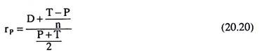
If D, r_P, T and n are known, then from (20.20) we would be able to know the value of P.

Irredeemable Preference Shares:

The owner of the irredeemable preference shares never gets back his money that has been invested. However, he gets dividend at a fixed rate perpetually.

Therefore, if the price of the share be P (Rs) and the amount of dividend per year for each share be D (Rs) = constant and if the cost of the share be r_P (Rs), then we obtain:

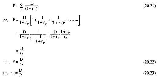
That is, if we know P and D, we would be able to know from (20.23) the cost of an irredeemable share (r_p). Again, if we know D and r_P, we would be able to know the value of P from (20.22).

Concept # 7. Cost of Retained Earnings (or Internal Equity):

Undistributed profits are the un-obtained dividends of the owners of shares. The rate of return that the owners of ordinary shares could have obtained from these un-obtained dividends, is itself the cost of undistributed profits.

We may find the rate of return that the owners of ordi­nary shares could obtain with the help of the Dividend Capitalisation Approach (DCA).

From equation (20.13) we obtain this rate of return (r_e) as:

r_e=D_L /P₀ + g

where D₁ = annual dividend of each share in the first year

g = annual rate of increase of dividend (= constant, assumed)

P₀ = present value of each share

Now, if the undistributed profits are distributed as dividends among the shareholders, then with this money, they can buy the shares of this company or they can buy the shares with similar risk of some other companies and they may get a rate of return equal to r_e.

Therefore, by investing the undistributed profits, the firm would have to earn return at a rate equal to r_e, so that an increase in the share price and in the amount of dividend could be ensured. If the rate of return from the investment of undistributed profits be less than r_e, then the price of the firm’s share would be diminishing.

Therefore, the rate of return that the owners of firm’s shares might obtain, would itself be the cost of undistributed profits.

That is, we obtain:

Cost of undistributed profits (r_r) = r_e                                     (20.24)

Concept # 8. The Composite or Overall Cost of Capital:

The firms generally maintain a pattern or structure of different types of capital. For example, a company may be willing to maintain a structure like this: 30 per cent of its total capital raised as loan capital and 70 per cent as equity capital. Again, another company may maintain a pattern of 60 per cent of loan capital and 40 per cent of equity capital.

The capital structure of a company would depend upon the nature of its business and its willingness to bear risk. The natures of some businesses are such that the firms do not hesitate to take risk.

For example, the public utility companies, since they enjoy a monopoly power in the market, may be willing to bear a lot of risk. Because, they know that their products are essential commodities and so their sales, income and profit flows are stable and secure.

On the other hand, there are companies that enter into more risky ventures because they think that the more the risk, the more would be the profit. The companies that are able to, or willing to, take more risk, have a greater share of loan capital in their capital structure, because they do not mind facing the commitment to pay more in the form of interest or principal repayment.

On the other hand, there are companies that want to avoid taking too much of risk, and so, they maintain a relatively smaller share of loan capital and a relatively larger share of equity capital in their capital structure.

If a company wants to maintain a particular pattern in its capital structure, then, in order to evaluate each of a number of investment projects, it uses an overall or composite cost estimate of different types of capital as one of the criteria—it does not associate each project with a particular type of capital and its cost.

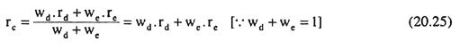
This composite cost of capital (r_c) is a weighted average of net cost of loan capital (r_d) and the cost of equity capital (r_e). Here the proportion of loan capital in the firm’s total capital (w_d) and the proportion of equity capital (w_e) are taken as the respective Weights of r_d and r_e.

We therefore have: