
The following points highlight the top four models of Aggregate Supply of Wages. The Models are: 1. Sticky-Wage Model 2. The Worker Misperception Model 3. The Imperfect Information Model 4. The Sticky-Price Model.
Aggregate Supple Model # 1. Sticky-Wage Model:
The proximate reason for the upward slope of the AS curve is slow (sluggish) adjustment of nominal wages.
In most organised industries nominal wages are set for a number of years on the basis of long-term contracts.
So wages do not move up or down whether the economy speeds up or slows down.
ADVERTISEMENTS:
The range of wage movements is also narrow in those industries not covered by formal contacts due to implicit agreements between employees and employers. Wages may also depend on conventions, or social norms as the classicists like David Ricardo had postulated, as also on the concept of justice (fairness) that evolves over time. For all these reasons nominal wages are taken as sticky in the short run.
The following three things happen to aggregate output when the price level rises:
1. When the nominal wage is stuck, a rise in the price level lowers the real wage, reducing the real cost of labour.
2. This induces firms to hire more labour.
ADVERTISEMENTS:
3. As a result output increases.
Thus there is a positive relationship between the price level and the amount of output produced. This means that the AS curve is upward sloping even when the nominal wage cannot adjust.
Here we assume that workers and firms voluntarily agree to accept a particular nominal wage on the basis of collective bargaining. They do not know at this stage what the price level will be when the wage agreement becomes effective.
Both the parties have in mind a target real wage, which is likely to be higher than its market clearing level for two reasons:
ADVERTISEMENTS:
(i) the bargaining power of trade unions, and
(ii) efficiency-wage considerations.
The employees and employers set the nominal wage (W) on the basis of the target real wage (w) and the expected price level (Pe):
W = w.Pe … (2)
After setting the nominal wage and before hiring labour, firms come to know exactly what the actual price level (P) is.
So the real wage turns out to be:
W/P = w.Pe/P … (3)
The real wage is nominal wage times the ratio of the expected price level to actual price level.
This implies that the real wage deviates from its target if the actual price level deviates from its expected level:
ADVERTISEMENTS:
(i) when P > Pe, W/P < w
(ii) when P < Pe, W/P > w
Finally we assume that the level of employment is determined by the firms’ demand for labour at the predetermined wage, and not by a collective bargaining process.
The demand function for labour is expressed as
ADVERTISEMENTS:
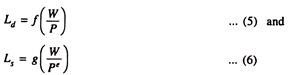
Ld = f(W/P) where f'(W/P) < 0 …(4)
which means that the lower the real wage, the higher is the demand for labour by firms. The level of output is determined by the production function
Y = F(L)
The more labour is hired, the more output is produced.
ADVERTISEMENTS:
Fig. 13.2 shows how the AS curve is derived from the labour demand curve and the aggregate production function.

Watch the Sequence and Note the Causation:
1. An increase in P in part (c) reduces (W/P) in part (a).
2. A fall in (W/P) raises employment in part (a) and (b) from L1 to L2.
3. As a result Y increases in part (b) and part (c) from Y1, to Y2.
ADVERTISEMENTS:
4. The direct relation between P and Y is captured by the AS curve of part (c).
The demand curve for labour is shown in part (a) of Fig. 13.2. Since the nominal wage W is stuck, an increase in the price level from P1 to P2 reduces the real wage from (W/P1) to (W/P2). The lower real wage increases labour demand from L1 to L2.
The corresponding aggregate production function is shown in part (b). An increase in the quantity of labour demanded raises output from Y1, to Y2 Part (c) shows that an increase in the price level from P1 to P2 raises output (and income) from Y1 to Y2.
The locus of alternative combinations of P and Y is the AS curve which is expressed by the following equation:
Y = Y̅ + α(P – Pe)
In short, since the nominal wage is sticky, an unexpected change in the price level (P ≠ Pe) causes a deviation of the real wage (W/P) from its target level (w). This change in (W/P) affects the amounts of labour hired and output produced.
Aggregate Supple Model # 2. The Worker Misperception Model:
ADVERTISEMENTS:
The worker misperception (fooling) model, presented by Friedman in 1968 (in his article entitled “Role of Monetary Policy”, American Economic Review) is based on the assumption that wages can adjust freely and quickly to equilibrate the labour market.
Since workers temporarily equate a rise in nominal wage to a rise in real wage, i.e., they suffer from money illusion, unexpected movements in the price level influence labour supply. In this model, while the quantity of labour demanded by firms depends on the actual real wage, the quantity of labour supplied depends on the expected real wage, which is nominal wage (W) deflated by the expected price level (Pe), i.e.,
The reason for this is that while deciding on how much labour to supply, workers know their nominal wage but not the overall price level (P). Expected real wage can be expressed as the product of actual real wage and a new variable P/Pe:
![]()
Here, P/Pe measures workers’ misperception of the price level. If the value of this new variable exceeds 1, then P > Pe, i.e., actual price exceeds the expected price. If P < Pe, the converse is true.
ADVERTISEMENTS:
Now, if we substitute equation (7) in equation (6) we get:
![]()
This means that the quantity of labour supplied depends on the real wage and on worker misperception of the price level. According to this model, an unexpected rise in the price level makes workers feel that the real wage has gone up. But this is a false belief.
Living in a world of illusion they are induced to supply more labour at the initial real wage. This reduces the real wage from (W/P)1 to (W/P)2 in Fig. 13.3 and raises the demand for labour from L1 to L2. The end result is a rise in employment, output and income.

Even in this model, where workers believe (in the event of a rise in overall price level) that the real wage is higher than it actually is, deviations of actual prices from their expected levels induce the workers to increase their supply of labour. This, in its turn, alters the output levels of firms.
ADVERTISEMENTS:
So the equation of the short-run aggregate supply (SRAS) curve is the same as in the sticky-wage model:
Y = Y̅ + α(P – Pe)
or, Yg = Y – Y̅ = a (P – Pe).
The actual output deviates from its natural rate when the actual price level deviates from the expected price level. Here Yg measures the output gap.
Aggregate Supple Model # 3. The Imperfect Information Model:
The basic assumption of the imperfect-information model is that all wages and prices are market-determined rather than bargain-determined. They are free to adjust in response to forces of demand and supply in labour and commodity markets.
In this model, short-run and long-run aggregate supply curves differ because of temporary misperceptions about movements in absolute and relative prices. See Fig. 13.4. In Fig 13.4(a) we show changes in relative prices such as Pb/Pa, Pc/Pa, Pd/Pa, Pc/Pb, Pc/Pd etc. In Fig, 13.4(b) we show the differences between a once-and-for-all price rise and a sustained or continuous price rise (inflation).

The imperfect-information model is based on the assumption that each supplier in the economy produces a single good and consumes many goods. Since innumerable goods are produced in an economy, it is virtually impossible for suppliers to observe all prices at all times. It has to be noted that suppliers of certain goods are consumers of other goods, i.e., they are both sellers and buyers.
They keep a close watch on the prices of the products they sell, but it is not possible for them to closely watch the prices of the goods they buy for consumption purposes. Due to imperfect information, they fail to understand the difference between inflation or deflation (which refers to the rise or fall in the overall price level) and price movements (changes in relative prices).
This confusion influences decisions about how much output to offer for sale and a positive relation is established between the price level and output in the short run.
In case of unanticipated inflation, all the suppliers find that the prices of their goods are rising at the same time. They all predict rationally, but wrongly, that the relative prices of the goods they produce have risen. So they work harder and produce more. Since the actual prices exceeded their expected levels, suppliers raise their output.
So the aggregate supply curve, which is expressed by the equation Y = Y̅ + α(P – Pe), slopes upward from left to right. So, in this model also, Y deviates from Y̅ when P deviates from Pe.
Aggregate Supple Model # 4. The Sticky-Price Model:
The sticky-price model has a micro-foundation. It is based on the pricing behaviour of firms in large oligopolistic markets. In oligopoly, we normally find output fluctuations in the face of fluctuating demand; we do not find short-run price adjustments when demand changes. Frequent price changes create confusion and annoyance among regular buyers.
There is loss of goodwill. Moreover, there is the cost of changing prices. New prices are to be printed, they are to be announced through newspapers and TV commercials and new catalogues are to be distributed to retailers all over the country. These are all costly affairs in terms of time lost and money spent.
The sticky price model is based on the assumption that firms have some monopolistic or oligopolistic control over the prices of their products. So we deviate from the model of perfect competition where a firm is a price-taker.
A typical firm’s desired price p depends on two macroeconomic variables:
(i) The aggregate price level (P) which is a weighted average of all individual prices: A high P implies that the firm’s costs are higher. Hence higher the P, higher will be the price of the product of any firm.
(ii) The national income of the country (Y): A higher level of income widens the market for a firm’s product. Since marginal cost increases with an increase in the volume of production, the greater the demand, the larger the volume of production, and the higher the firm’s desired price.
The firm’s desired price is expressed as:
p = P + α(Y- Y̅) … (9)
This means that the desired price p depends on the general price level and the divergence of actual output from its level (potential/natural). The parameter a, which is positive, measures the degree of responsiveness of a firm’s desired price to the level of aggregate output.
Diverse Price Behaviour:
Let us assume that there are two types of firms. Some have flexible prices, because they set prices according to equation (9). Others have sticky prices, in the sense that they announce their prices in advance on the basis of their expectation about future economic conditions, i.e., on the basis of whether they expect the economy to speed up or slow down.
The price-fixing strategy of firms with sticky prices is expressed by the following equation:
p = Pe + α(Ye – Y̅e) …(10)
where the superscript V denotes the expected value of a variable. If we assume, for the sake of simplicity, that these firms expect actual output to be at its natural rate, then the last term, a(Ye – Ye), disappears. Then these firms set the price
p = P*…(11)
This means that firms with sticky prices set their prices on the basis of what they expect Other firms to charge.
If we are to derive the AS curve we have to find out the overall price level in the economy, by making use of the pricing rules of the two groups of firms. If k is the proportion of firms with stick prices, then the overall price level is
P = kPe + (1 – k) [P + α(Y – Y̅)] … (12)
Here kPe is the price of the sticky-price firms weighted by their proportion in the economy and the second term in equation (12) is the price of the flexible-price firms, weighted by their proportion. If we now subtract (1 – k)P from both sides of equation (12) we get
P – P + kP = kPe + (1 – k) P + (1 – k)a (Y – Y̅) – (1- k)P
or kP = kPe + (1 – k) [a(Y – Y̅)] … (13)
If we divide both sides by k,. we get the overall price level
P = Pe + [(1 – k) a/k] (Y – Y) … (14)
The terms in this equation may now be explained:
(i) When firms expect a high price level, they expect high costs, too. Those firms that fix prices in advance set prices at high level in anticipation of high costs. This means that expectations of firms come true. A high expected price level Pe leads to a high actual price level P.
(ii) When Y is high, the demand for goods is also likely to be high. So firms with flexible prices fix their prices at high levels. As a result the general price level goes up. Now the effect of output expansion on the general price level depends on the proportion of firms with flexible prices.
Thus we see that the overall price level depends on the expected price level and on the level of output. Now we can show the equivalence of the aggregate pricing equation (14) and the equation of the aggregate supply curve (1).
Equation (14) can be expressed as:

Thus we convert the aggregate pricing equation into the standard form of the aggregate supply equation, presented in three other models. Thus the sticky price model also suggests that the deviation of output from tits full employment level is directly related to the price deviation factor (P – Pe).
The Effect on the Labour Market: Cyclical Behaviour of Real Wage:
No doubt the sticky-price model emphasises the goods market. But we can also analyse the implication of the model on the labour market. If a firm’s price is stuck in the short run, then a fall in aggregate demand reduces the sales level of the firm. So a fall in production is inevitable.
This will automatically reduce the demand for labour. By comparison, in the sticky-wage model, the firm does not move along a fixed labour demand curve. Rather fluctuations in output are associated with shifts in the labour demand curve. And employment, production, and the real wage are all likely to move in the same direction as a result of such shifts in labour demand.
Thus the real wage is likely to be procyclical. It is likely to rise in prosperity and fall in depression.
The four models of aggregate supply are not incompatible with one another. They are not mutually exclusive either. Since the real world may contain all the four types of imperfections or frictions we cannot accept one model and reject the other three.