The Transactions Demand for Money: A Close Look

The Transaction Demand for Money:

A third approach to the demand for money is the inventory approach to transactions demand developed by both Baumol and Tobin. They show that there is a transactions need for money to smooth out the difference between income and expenditure streams, and that the higher the interest rate — the return on holding bonds instead of money — the smaller these transactions demand balances should be.

Transactions theories emphasise the role of money as a medium of exchange.

These theories highlight two important points:

(i) Money is a dominated asset;

(ii) People hold money, unlike other assets, to make purchases.

These theories seek to explain why people hold narrow measures of money M₁, such as currency and deposits withdrawable by cheques, as opposed to holding assets that denominate them, such as savings accounts or Treasury Bills.

There are various theories of transactions demand for money. They differ from one another to some degree depending on the process of obtaining money and making transactions. But all these theories have a common theme they suggest that money has the cost of earning a low rate of return and the benefit of making transactions more convenient. People face a trade-off between these costs and benefits while deciding how much money to hold for carrying out the required number of transactions per period. In this context, we refer to the Baumol-Tobin model and see how the model explains the money demand function.

Keynes’ theory of the transactions demand for money has been extended by Baumol and Tobin by following an important theory of management called inventory-theoretic approach.

The transactions demand for money has been treated as the inventory of the medium of exchange (money) that will be held by an individual or a firm. This theory of the optimal level of the inventory has been developed along the lines of the theory of the inventory holdings of goods by a firm.

One of the reasons that households and business firms hold currency and keep funds in their chequing account is the same as the reason stores keep inventories of goods for sale. Since income is received periodically and expenditures occur regularly, it is necessary to hold stock of currency and deposits withdrawable by cheques.

This is the essence of Baumol’s inventory theory of the demand for money which is an extension of the Keynesian theory of transactions demand for money. Baumol’s approach was extended by James Tobin. Here we present a simple version of the Baumol-Tobin model.

The Baumol-Tobin Model:

The Baumol-Tobin model is based on a formula called the square-root rule. This is akin to the square-root rule for inventories. The square-root rule says that stores should hold inventories proportional to the square-root of sales. The same square-root rule applies to the demand for money also.

The square-root rule gives a household’s transactions demand for cash. According to this rule, the household holds less money if the opportunity cost of holding money or the rate of interest (i) increases. The service of money is akin to anything else the household consumes.

It consumes less when the price level rises. The square-root rule also says something about the relation between total spending and income (Y) and the household’s demand for money. The demand depends on the square-root of total income. In comparing two families, one with double the income of the other, we should find that the second family has a transactions balance only 41% higher (the square root of 2 is 1.41). The inventory-theoretic approach to the transactions demand for money provides a theoretical basis for the inverse relationship between demand for money and the interest rate.

The Baumol-Tobin model brings into focus, in an apt analytical way, the costs and benefits of holding money. The benefit of money holding is the convenience people want to enjoy from the most liquid of all assets. People hold money to avoid going to the bank every time they want to buy something.

At the same time money holding is costly. It costs money to hold money and the rate of interest is the opportunity cost of money holding. By holding money, people lose the opportunity to earn interest, i.e., the forgone interest they would have received had they left the money deposited in a savings account, or fixed deposit.

To see how people trade off these benefits and costs, let us consider a person who plans to spend Rs Y gradually over a year. (Here we assume that the price level is constant which means that real spending is also constant over the year).

The question here is: what is the optimal size of his average cash holdings? Or, to put the question in a different language, how much money should he hold in the process of spending this amount?

Three Possibilities:

Here we consider three possibilities. He could withdraw the whole amount (Y) at the beginning of the year and spend it gradually. In Fig. 19.7, we show that average money holdings depend on the number of trips a person makes to the bank each year. Fig. 19.7(a) shows his money holdings over the course of the year, under this plan.

His money holding at the beginning of the year is Y and at the end of the year is zero. So his average money holding (cash balance) is Y/2 over the year.

The second possible plan is to make two trips to the bank per annum, in which case he withdraws Y/2 rupees at the start of the year, gradually spends this amount over the first half of the year, and then makes another trip to withdraw Y/2 for the second half of the year. Fig. 19.7(b) shows that money holdings over the year vary between Y/2 and zero.

So average money holding (cash balance) in this case is 174. This plan has the advantage that less money is held on average. So the individual forgoes less interest. But it has the disadvantage of requiring two trips to the bank instead of only one.

Now we may consider a more general situation where an individual makes N trips to the bank over the course of the year. Every time he makes a trip, he withdraws Y/N rupees. He then spends the money gradually and evenly over the following 1/N^th of the year. Fig. 19.7(c) shows that money holdings vary between Y/N and zero, averaging Y/(2N).

Optimal choice:

What, then, is the optimal choice of N? The greater N is, the less money the individual holds on average and the less interest he forgoes. But, as N increases, the individual faces greater inconvenience. He has to make frequent trips to the bank.

Let the cost of going to the bank be a fixed sum F, which represents the value of the time spent travelling to and from the bank and standing in queue to withdraw cash. The interest rate is denoted as i, which is the opportunity cost of holding money.

Now we may analyse the optimal choice of N, which determines money demand. For any N, the average amount of money held is Y/(2N). So the forgone interest is iY/(2N). Since F is the cost per trip to the bank, the total cost of making trips to the bank is FN.

So the total cost (C) of an individual is:

C = forgone interest + cost of trips

= iY/(2N) + FN … (10)

The larger the number of trips N, the smaller the forgone interest, and the higher the cost of going to the bank.

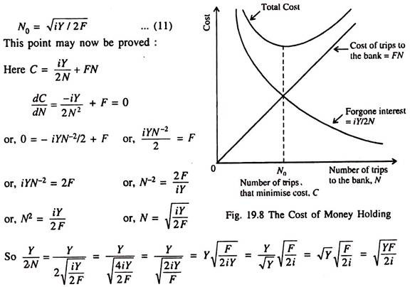
Fig. 19.8 shows how C depends on N. There is only one value of N which minimises C. The optimal value of N, denoted as N₀, is

Thus, average money holding is Y/2N₀ =  . This expression shows that the individual holds more money if the fixed cost of going to the bank (F) is higher, if income (Y) — on which his expenditure depends — is higher, or, if the interest rate i is lower.

Fig. 19.8 shows that forgone interest, the cost of trips to the bank, and the total cost depend on the number of trips N. Only one value of N, denoted as N₀, minimises total cost.

The Baumol-Tobin model explains the amount of money held outside of banks. But we can interpret the model more broadly. Let us suppose a person holds a portfolio of monetary
assets (currency and demand deposits) and non-monetary assets (stocks and bonds). Monetary assets can be used for transactions but they offer a low rate of return.

Let i be the difference in the return between monetary and non-monetary assets, and let F be the cost of transferring non-monetary assets into monetary assets, such as brokerage fee. The decision about how often to pay the brokerage fee is quite similar to the decision about how often to make a trip to the bank.

Therefore, the Baumol-Tobin model describes a person’s demand for monetary assets. By showing that money demand depends positively on expenditure (K) and negatively on the nominal interest rate (i), the model provides a microeconomic rationale for the Keynesian money demand function (M/P)_d = f(Y, i)

Implication:

One major implication of this model is that money being the medium of exchange there is some cost involved in transforming interest-earning assets into money, that there is a brokerage fee, which is denoted here as the number of trips to the banks (N). The value of N is the crucial variable in Baumol-Tobin model.

The role it plays in the model is that of any cost in selling income-earning assets; this could just as well be the time and trouble taken by an individual to sell an asset himself as anything else. So any change in the fixed cost of going to the bank F alters the money demand function, that is, it changes the quantity of money demanded for any given interest rate and income.

The spread of modern technology such as use of automatic teller machines, for instance, reduces F by reducing the time it takes to withdraw money. Likewise, the introduction of internet banking reduces F by making it easier to transfer funds among accounts. In contrast, an increase in real wages increases F by increasing the value of time. Likewise an increase in banking fees increases F directly. Thus, although the Baumol-Tobin model gives us a very specific money demand function, it does not give us any reason to believe that this function will necessarily be stable over time.

Some individuals and households keep their wealth in the form of money. They sometimes have large amounts in their chequing accounts at zero or low interest rates.

Keynes’s notion of speculative demand for money no doubt fits into this store-of-wealth category. The speculative demand captures the idea that changes in market interest rates will change the value of bonds. For individuals bonds paying fixed interest rates are one of the main alternatives to holding money in financial institutions. But, when interest rates rise, market prices of old bonds fall.

Keynes argued that when interest rates were high; more people would expect them to fall or, equivalently, would expect bond prices to rise and would, therefore, want to hold more bonds and less money. Thus the demand for money falls with a rise in interest rates. Changes in bond prices add risks to holding bonds. People are assumed to be risk-averse. So they are reluctant to put all their wealth in one risky asset.

Some of their wealth will be held as relatively riskless money. Unless they are unwilling to assume any risk, they will balance wealth between money and bonds. This act of balancing gives rise to a demand for money as an aversion to risk, as has been suggested by Tobin who extended the Keynesian theory of speculative demand for money.

The second implication of the model is that for the economy as a whole, the demand for money will depend on the distribution of income as well as upon its level. Finally, the model predicts that the demand for money will increase in less than proportion to the volume of transactions, that there are economies of scale in money holding for the individual.

So monetary policy might prove to be more powerful than what Keynes had suggested. With a given distribution of income, any increase or decrease in the supply of money will have a bigger effect on the level of income in situations of unemployment than it would be if the demand for money were proportional to the level of income.

However, the empirical studies of demand for money available so far provide little clear support for the transactions cost approach. In addition, the inventory approach is open to the general theoretical objection that it takes the pattern of payments and receipts as given whereas these patterns can be construed instead as an optimising response to the social usefulness of money as a medium of exchange and store of value.

Interest Elasticity of Transactions Demand for Money:

We know that one principal motive for holding money is the need to smooth out the difference between flows of income and expenditure. This transactions motive lies behind the trans­actions demand for money which is related to the level of income. The alternative to holding money, which is the means for payments and earns no return, is bonds, which earns a return but also involve transactions costs — brokerage fees — as one moves from money (received as pay) to bonds and back to money to make expenditures. The higher the interest rate bonds earn the tighter transactions balances should be reduced to hold bonds — making the transactions demand for money slightly sensitive to interest rate changes.

Let us suppose an individual is paid monthly (in cash or by cheque) and spends the total amount C of his income in purchases spread evenly throughout the month. He has the option of holding transactions balances in money or in bonds which yield a given i, i₀, if held for a month, and proportionately less than i₀ if they are held for a shorter period.

The individual would prefer to hold bonds since they yield a return but will have to convert bonds to cash during the month to meet expenditure plans. The first question we want to ask is: How frequently should he convert bonds into cash? That is: How many bonds-to-cash transactions should he plan, where N is the number of these transactions?

To begin on the revenue side, if an individual plans no bonds-to-cash transactions, he buys no bonds in the first place. In this case, then he can hold no bonds during the period and would earn zero return. Next, suppose he plans one bonds-to-cash transaction, putting half of C into bonds which he holds half the month. In this case total revenue R from interest will be i₀/2 times C/2, or (i₀C)/4, as shown in Table 19.1. Marginal revenue (MR) from the increase in transactions from zero to one is also (i₀C)/4.

If two transactions are planned, two-thirds of C can be put into bonds initially. For every ten days of the month, half the bonds (or, 1/3 of C) can be cashed. Each bond will have earned i₀/3, giving revenue on this third of C equal to (i₀C)/9. Ten days later the other half can be cashed having earned 2i₀/3 per bond or (2r₀C)/9 revenue for this third of C. Total revenue in the two-transaction case will then be (i₀C/9 + (2i₀C)/9 = (i₀C)/3. The increase in revenue, MR, over the one-transaction case is (i₀C)/12, as shown in Table 19.1.

In the three-transaction case, one-fourth of C will earn interest for one-fourth of the month, yielding (i₀C)/16; one-fourth will earn for half the month, yielding (2i₀C)/16; and the final one-fourth (½) will earn interest for three-quarters of the month, yielding (3i₀C)/16. The total revenue in this case is (6i₀C)/16, or (3i₀C)/8. MR in the three-transaction case is (i₀C)/24.

So the marginal revenue from increasing the number of transactions is positive and decreasing as the number of transactions N increases. Furthermore, as N increases the drop in MR decreases. This is why the MR(i₀) curve in Fig. 19.9 shows MR as a function of the number of transactions N for the given initial interest rate i₀.

On the cost side, we assume each transaction has a given cost tC, perhaps a broker’s fee or the implicit cost of time spent in transacting business. Then we can add a (marginal cost) MC = tC schedule to Figure 19.9. Com­bined with the initial MR(i₀) curve, this gives a profit-maximising number of transactions N₀ where MR = MC.

For any given number of transactions, such as N₀ in Fig. 19.9, an increase in the expen­diture flow C will increase average holdings of both money and bonds during the month. If the expenditure flow is smooth, so that total trans­actions balances of B + M equal C at the beginning of the month and zero at the end, then the average total holding is C/2. The number of transactions tells us how that C/2 is split between money and bonds. Thus, an in­crease in expenditure, or in general an increase in the flow of real income and output Y, will raise the transactions demand for money.

From the example in Table 19.1, it is quite clear that an increase in the number of transactions increases the average bond holding during the month and decreases the average money balance. At one extreme, with zero transactions, no bonds are held and the average money balance equals C/2. With a very large number of transactions, very little money is held, and average bond holdings approach C/2.

Now the MR curve in Fig. 19.9 is positioned by a given interest rate i₀. The MR entries in Table 19.1 all have i in their numerators, so an increase in i from i₀ to i₁ will increase MR for any given number of transactions, shifting the MR(i₀) curve up to MR(i₁) in Fig. 19.9. With no change in the cost per transaction, this increases the optimum number of transactions to N₁. The increase from N₀ to N₁ is made in order to increase average bond holdings to take advantage of the higher i.

Thus, an increase in the interest rate should reduce the transactions demand for money for any given level of the income-expenditure stream. So the demand-for-money function is M_d/P = L_i + kY.

The transactions demand for money should respond to a change in the interest rate through a change in the number of bonds-to-money conversions. The speculative demand should respond to a change in i due to portfolio-balancing considerations. Both effects together lead to fall in the demand for real balances (M_d/P) as i increases.

Changes in Transactions Demand for Money:

There may be changes in transactions demand for money for various reasons.

The following four factors have practical relevance in the context of Baumol-Tobin model:

(i) Effects of income redistribution:

If income is more equitably distributed, say, through tax-subsidy measures, the total expenditure of the people of a country is likely to increase. As a result the aggregate transactions demand for money will increase. Those who pay taxes are unlikely to reduce their transactions demand for money much. But those who receive subsidy will demand more money for transactions purposes because they have a strong propensity to consume. These people do outnumber the taxpayers. So the total transactions demand for money will increase.

(ii) Effects of vertical integration:

A vertical integration (merger) combines two firms that previously had an actual or potential customer-supplier relationship. This means that the product of one firm is used as an input by the other firm. An example of this is the merger of a manufacturer of computers with a producer of electronic components. A vertical merger replaces a market transaction by an intrafirm transaction.

Vertical integration eliminates the costs of transactions but also involves higher costs in coordinating two distinct operations. So it is not possible to predict whether vertical integration will lead to a fall or a rise in the transactions demand for money.

On the other hand the demand for cash will fall due to intrafirm transaction. If, for instance, a steel plant acquires an iron ore mine, the former need not pay cash every time it buys iron ore. At the same time more expenditure has to be incurred to coordinate the activities of an input-supplying firm with an output-producing firm.

(iii) A wave of credit card fraud:

If there is a wave of credit card fraud the transactions demand for money will initially increase. This means that the LM curve will shift to the left and the rate of interest will rise. This may, ultimately, reduce transactions demand for money.

(iv) Introduction of monthly payments system:

The transactions demand for money also depends on the method of wage payment, i.e., with the frequency with which wages are paid.

A daily wage earner does not hold much transactions balance. He earns wage income every day and spends it immediately. He may keep some precautionary balance so that he can manage to survive if he falls sick and is unable to work for a few days. In India wages are usually paid on a monthly basis. But in Britain wages are paid on a weekly basis.

So an average British worker holds less transactions balance (as a proportion of his income) compared to an average Indian worker. Now if the weekly system of wage payment is replaced by a monthly payment system, transactions demand for money will definitely increase.

Policy Implications of Interest Elasticity of Transactions Demand for Money:

In Ch. 8 we noted that when the speculative demand for money is infinitely elastic with respect to i as during depression, monetary policy loses its effectiveness completely. But monetary policy becomes more and more effective as the interest elasticity of the demand for money increases. This point is explained by referring to Baumol-Tobin model where

where M_s is money supply, M_d is money demand, i is the interest rate and N is the number of trips to the bank. If Y is to be increased by 4 times money supply has to be doubled (if money market equilibrium is to be maintained):

This implies doubling money supply increases Y four times. This is in sharp contrast to the prediction of the quantity theory of money which suggests that a doubling of money supply (M_s) will double Y.

This is a very interesting result: interest elasticity of money supply makes monetary policy more powerful. This means that if the demand for money is interest-elastic, the supply of money will have to be adjusted accordingly to maintain money market equilibrium. In other words, money supply has to be elastic too, which calls for sufficient flexibility in the central bank’s monetary policy. Such a policy will increase the value of the money multiplier (a concept to be discussed in a next chapter) and make monetary policy more effective than if the transactions demand for money is not interest elastic.

If transactions demand for money is elastic with respect to the rate of interest monetary policy becomes effective. This conclusion is in sharp contrast with the one which is derived when the speculative demand for money is fairly elastic. When the speculative demand for money is completely elastic at a particular rate of interest (the liquidity trap case) monetary policy is completely powerless in influencing the macro-variables.

The Quantity Theory as a Theory of Demand for Money:

Modem quantity theorists treat the demand for money in just the same way as the demand for any other financial or physical asset. In consumption theory the demand for a good is determined by its attributes, including its price in relation to other goods, the purchaser’s set of choices being subject to an income constraint.

Similarly, in asset theory the demand for any particular asset is determined by its characteristics including its yield in relation to that of other assets — the asset-holder’s set of choices being subject to a wealth constraint. However, as A. D. Bain said: “The problems encountered in specifying demand functions for financial assets, including money, are no different in their essentials from the problems of consumer-demand analysis.”

Friedman’s Restatement:

Friedman, in fact, restated the Quantity Theory as a theory of demand for money (or velocity) and not a theory of prices or output, and made the essence of the theory the existence of a stable functional relation between the quantity of real balances demanded and a limited number of independent variables, a relation deduced from capital theory.

However, as Don Patinkin has argued: “What Friedman has actually presented is an elegant exposition of the modern portfolio approach to the demand for money which can only be run as a continuation of the Keynesian theory of liquidity preference.” However, the restated quantity theory introduces wealth constraint and emphasises expected changes in the price level as an element in the cost of holding money and other assets fixed as to both capital value and yield in money terms, whereas Keynesian portfolio balance theory almost invariably starts from the assump­tion of an actual or expected stable price level.

Friedman’s restatement obtained the immediate tacit advantage of freeing it from the Keynesian criticism of assuming an automatic tendency towards full employment in the economy, by making it a theory of the demand for money without commitment to the analysis of prices and employment.

Friedman argues that money can be regarded as one of five broad ways of holding wealth: money, bonds, equities, physical goods and human wealth. Each of these has distinctive characteristics and each offers some return in money or in kind.

The yield on money is mainly in kind — a convenience yield which reflects trouble and transaction costs which can be avoided if ready money is available — though, as some forms of money, e.g., saving deposits in banks, also have an explicit money yield. The real, as opposed to nominal, yield on money depends on movements in the price level. If the price level falls, money appreciates and shows a capital gain in real terms which must be added to the nominal yield, while in the more common condition of rising prices a real capital loss has to be deducted from the nominal yield.

Bonds stand for assets which promise a perpetual income stream of constant amount. Like money, their real return is affected by changes in the price level, but it is also affected by changes in the rate of interest on bonds. If the rate of interest on bonds is r_b, the nominal rate of return can be approximated by

r_b – (1/r_b). (dr_b)/(dt)

where (1/r_b).(dr_b)/(dt) measures the rate of capital appreciation due to change in the rate of interest.

Equities stand for assets which promise a perpetual income stream of constant real amount. If the rate of interest on equities is Rs r_e and if prices are stable, the nominal rate of return is affected both by changes in this rate of interest and by changes in the price level. The associated changes in capital value can be approximated by -(1/r_e)(dr_e)(dt) and (1/P)(dP)/(dt), respectively. So the nominal rate of return must also take account of the price level P.

Physical goods yield an income in kind which can seldom be measured by any explicit rate of interest. Their nominal rate of return is, however, also affected by the rate of change of the price level (1/P)dP/dt which can be considered explicitly. Human wealth is the discounted value of the expected stream of earned income. It presents a problem because it can be substituted only to a very limited extent with other forms of asset holding.

Nevertheless some substitution is possible: people cart sell assets in order to pay for training which will increase their future earnings and their expected earnings also influence the amount which they can borrow and hence their gross asset holdings. In principle the limitations on substitutability make a case for distinguishing between human and non-human wealth in the demand function, which can be done by including in it the ratio of non-human to human wealth, w.

Finally, the wealth constraint must enter the demand function. In the absence of direct estimates of wealth, including human wealth, an indirect estimate must be used. Friedman makes use of permanent income Y_p — a weighted average of current and past values of income-as an indicator. Some other investigators have confined the constraint to non-human wealth, W.

This adds up to a formidable list of factors which should enter into the demand function for money:

There will also, of course, be differences in individual demand functions due to differences in preferences, u.

For empirical work, further simplifications must be made. First, if we follow the Keynesian logic of the speculative demand for money, the relevant capital gains on bonds and equities are not found to be simply those which take place in practice but those which are expected to take place. No measures of expected capital gains or losses due to changes in interest rates are available, so these terms are usually dropped from the demand function.

The rate of change of prices has also usually been omitted, except in studies of hyperinflation, and the ratio of non-human to human wealth has seldom been included. Finally, for statistical reasons, investigators have usually had to be content with employing one rate of interest as an indicator instead of including the yields on a variety of financial assets simultaneously.

With these simplifications, the demand function can be written as:

M=f(P, r, Y_p, u)

with W substituted for Y_p in some instances.

From the above formulation it is pretty obvious that a proportionate increase in prices and in the money value of all assets other than money would result in a non-proportionate increase in the demand for money holdings. It is because the demand for money is thought to be a demand for real balances, i.e., it will be independent of the scale which is used to measure values.

Accordingly, the demand function for real balances is obtained by dividing throughout by P:

The major difference between Friedman’s approach and that of Keynes is the former’s emphasis on wealth as opposed to current income as a key decision variable and the omission of any unstable element, such as is implied by the speculative demand for money. However, the asset approach fails to suggest that the elasticity of the demand for money with respect to the rate of interest will become infinite at some positive rate of interest, that is, the Keynesian liquidity trap.