Equilibrium of the Firm: Short-Run and Long-Run

In this article we will discuss about the short run and long run equilibrium of the firm.

Short-Run Equilibrium of the Firm:

The short run is a period of time in which the firm can vary its output by changing the variable factors of production in order to earn maximum profits or to incur minimum losses. The number of firms in the industry is fixed because neither the existing firms can leave nor new firms can enter it.

Its Conditions:

The firm is in equilibrium when it is earning maximum profits as the difference between its total revenue and total cost. For this, it essential that it must satisfy two conditions: (1) MC = MR, and (2) the MC curve must cut the MR curve from below at the point of equality and then rise upwards.

The price at which each firm sells its output is set by the market forces of demand and supply. Each firm will be able to sell as much as it chooses at that price. But due to competition, it will not be able to sell at all at a higher price than the market price. Thus the firm’s demand curve will be horizontal at that price so that P = AR = MR for the firm.

1. Marginal Revenue and Marginal Cost Approach:

The short-run equilibrium of the firm can be explained with the help of the marginal analysis as well as with total cost-total revenue analysis. We first take the marginal analysis under identical cost conditions.

This analysis is based on the following assumptions:

1. All firms in an industry use homogeneous factors of production.

2. Their costs are equal. Therefore, all cost curves are uniform.

3. They use homogeneous plants so that their SAC curves are equal.

4. All firms are of equal efficiency.

5. All firms sell their products at the same price determined by demand and supply of the industry so that the price of each firm is equal to AR = MR.

Determination of Equilibrium:

Given these assumptions, suppose that price OP in the competitive market for the product of all the firms in the industry is determined by the equality of demand curve D and the supply curve S at point E in Figure 1 (A) so that their average revenue curve (AR) coincides with the marginal revenue curve (MR).

At this price, each firm is in equilibrium at point L in Panel (B) of the figure where (i) SMC equals MR and AR, and (ii) the SMC curve cuts the MR curve from below. Each firm would be producing OQ output and earning normal profits at the maximum average total costs QL. A firm earns normal profits when the MR curve is tangent to the SAC curve at its minimum point.

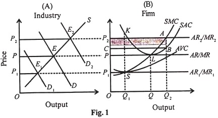
If the price is higher than these minimum average total costs, each firm will be earning supernormal profits. Suppose the price rises to OP₂ where the SMC curve cuts the new marginal revenue curve MR₂ (=AR₂) from below at point A which now becomes the equilibrium point. In this situation, each firm produces OQ₂ output and earns supernormal profits equal to the area of the rectangle P₂ ABC.

If the price falls below OP₁ the firm would make a loss because the SAC would be higher than the price. In the short-run, it would continue to produce and sell OQ₁ output at OP₁ price so long as it covers its AVC. S is thus the shut-down point at which the firm is incurring the maximum loss equal to SK per unit of output. If the price falls below OP₁ the firm will close down because it would fail to cover even the minimum average variable cost. OP₁ is thus the shut-down price.

We may conclude from the above discussion that in the short-run each firm may be making either supernormal profits, or normal profits or losses depending upon the price of the product.

2. Total Cost Revenue Analysis:

The short-run equilibrium of the firm can also be shown with the help of total cost and total revenue curves. The firm is able to maximize its profits at that level of output where the difference between total revenue and total cost is the maximum. This is shown in Figure 2 where TR is the total revenue curve and TC total cost curve.

The total revenue curve is an upward sloping straight line curve starting from O. This is because the firm sells small or large quantities of its product at a constant price under perfect competition. If the firm produces nothing, total revenue will be zero. The more it produces, the larger is the increase in total revenue. Hence the TR curve is linear and slopes upward.

The firm will maximize its profits at that level of output where the gap between the TR curve and the TC curve is the maximum. Geometrically, it is that level at which the slope of a tangent drawn to the total cost curve equals the slope of the total revenue curve.

In Figure 2, the maximum amount of profit is measured by TP at OQ output. At outputs smaller or larger than OQ between A and B points, the firm’s profits shrink. If the firm produces OQ₁ output, its losses are the maximum because the TC curve is above the TR curve. At Q₁ its profits are zero. Similar situation prevails at Q₂.

Since the marginal revenue equals the slope of the total revenue curve and the marginal cost equals the slope of the tan­gent to the total cost curve, it follows that where the slopes of the total cost and revenue curves are equal as at P and T, the marginal cost equals the marginal revenue. It should be clear that the point of maximum profits lies in the region of rising marginal cost (when TC is below TR) and of maximum loss in the falling marginal cost region (where TC is above TR).

The explanation of the equilibrium of the firm by using total cost-revenue curves does not throw more light than is pro­vided by the marginal cost-marginal revenue analysis. It is useful only in the case of certain marginal decisions where the total cost curve is also linear over a certain range of output.

But it makes the equilibrium of the firm a cumbersome and difficult analysis particularly when one has to compare the change in cost and revenue resulting from a change in the volume of output. Further, maximum profits cannot be known at once. For this, a number of tangents are required to be drawn which is a real difficulty.

Long-Run Equilibrium of the Firm:

In the long-run, it is possible to make more adjustments than in the short-run. The firm can adjust its plant capacity and scale of operations to the changed circumstances. Therefore, all costs are vari­able. Firms must earn only normal profits. In case the price is above the long-run AC curve firms will be earning supernormal profits.

Attracted by them, new firms will enter the industry and supernormal profits will be competed away. If the price is below the LAC curve firms will be incurring losses. As a result, some of the firms will leave the industry so that no firm earns more than normal profits.

Thus “in the long-run firms are in equilibrium when they have adjusted their plant so as to produce at the mini­mum point of their long-run AC curve, which is tangent (at this point) to the demand (AR) curve defined by the market price” so that they earn normal profits.

Its Assumptions:

This analysis is based on the following assumptions:

1. Firms are free to enter into or leave the industry.

2. All firms are of equal efficiency.

3. All factors are homogeneous. They can be obtained at constant and uniform prices.

4. Cost curves of firms are uniform.

5. The plants of firms are equal having given technology.

6. All firms have perfect knowledge about price and output.

Determination:

Given these assumptions, each firm of the industry will be in long-run equilibrium when it fulfils the following two conditions.

(1) In equilibrium, its short-run marginal cost (SMC) must equal to its long-run marginal cost (LMC) as well as its short-run average cost (SAC) and its long-run average cost (LAC) and both should be equal to MR=AR-P.

Thus the first equilibrium condition is:

SMC = LMC = MR = AR = P = SAC = LAC at its minimum point, and

(2) LMC curve must cut MR curve from below.

Both these conditions of equilibrium are satisfied at point E in Figure 3 where SMC and LMC curves cut from below SAC and LAC curves at their minimum point E and SMC and LMC curves cut AR = MR curve from below. All curves meet at this point E and the firm produces OQ optimum quantity and sells it at OP price.

Since we assume equal costs of all the firms of industry, all firms will be in equilibrium in the long-run. At OP price a firm will have neither a tendency to leave nor enter the industry and all firms will earn normal profit.