Top 4 Statistical Methods for Measuring Risk | Company

The following points highlight the top four statistical methods used for measuring risk. The methods are: 1. Probability 2. Expected Value 3. Variability or Dispersion 4. Standard Deviation (SD).

Statistical Method # 1. Probability:

If we toss an unbiased coin, we would obtain any one of two outcomes—head and tail. If we toss the coin quite a good number of times, we would obtain heads in about 50 per cent of the tosses and tails also in about 50 per cent of the tosses.

As the number of tosses increases and tends to infinity, the proportion of heads would tend to become equal to ½ and that of tails would also tend to become equal to ½. In this case, the probability of getting a head in a single toss of the coin is 50 per cent or ½ and that of getting a tail is also 50 per cent or ½.

We have to remember here that the sum of the probabilities of all the possible outcomes would be equal to 1. In the case of tossing a coin, we have ½ + ½ = 1.

We may take the help of another example to explain the concept of probability. Let us suppose that, from the shares of a company, a person has got 50 per cent dividend in 5 per cent periods, 30 per cent dividend in 60 per cent periods and 10 per cent dividend in 35 per cent periods. Here the three rates of dividend, viz., 50 per cent, 30 per cent and 10 per cent, are exhaustive. Therefore, in this case, probability of getting a dividend of 50 per cent is 5 per cent or 1/20, that of getting a dividend of 30 per cent or 12/20, and the probability of getting a dividend of 10 per cent is 35 per cent or

Statistical Method # 2. Expected Value:

In the above example, dividend is a variable ― its three exhaustive value are 50 per cent, 30 per cent and their probabilities are, respectively, In this case, the expected value of dividend is % or 24%. It is understood from the above example that the formula for expected value may be written in this way. If the values of a variable X are x₁, x₂,…,x_n with respective probabilities p₁, p₂,…,p_n, then the expected value of X would be

Statistical Method # 3. Variability or Dispersion:

The variability or dispersion of a variable is the extent to which its values are dispersed or scattered. For example, the first set of values of a variable are 30, 35, 40, 45 and 50, and a second set of values of the same variable are 5, 10, 30, 50 and 70. It is evident from these two sets of values that the variability of the second set is greater than that of the first set.

The significance of the variability being smaller or larger is very important. However, this significance is different in different cases.

For example, if the first set of values given above are the ‘runs’ of a particular cricketer in five different matches and the second set of values are the ‘runs’ in five matches of a second cricketer, then the significance of smaller variability in the first case and higher variability in the second case is that the first player is a more consistent performer than the second player.

Again, if the values of the first set are the rates of daily wages (in Rs) of five workers of a factory and the values of the second set are those of five workers of a second factory, then the fact that variability in the second case is larger signifies that the inequality of income among the workers of the second factory is larger than that in the first case.

Again, in a third field, if the values of the first set are the expected percentage rates of dividend to be obtained from the shares of a particular company and the values of the second set are those to he obtained from the shares of another company, then the fact that the values of the second set are more variable signifies that investment in shares of the second company is more risky than investment in the first company.

Similarly, if the rate of commission to be obtained from a job is more variable than that of a second job, then the income earnings from the first job is more uncertain than that from the second.

In some cases, variability may act as an index of risk. Therefore, in these cases, we may accept variability as a measure of risk.

Statistical Method # 4. Standard Deviation (SD):

Standard Deviation (SD) is the most widely used measure of variability. SD is defined as the positive square root of the expected value of the squares of the deviations of the values of a variable from its expected value or arithmetic mean.

Therefore, if the values of a variable, X, are x_]; x₂,. . ., x_n and their respective probabilities are f(x₁), f(x₂), . . ., f(x_n), and if the expected value of X be E(X), then the SD of the variable, X, is given by

 

 

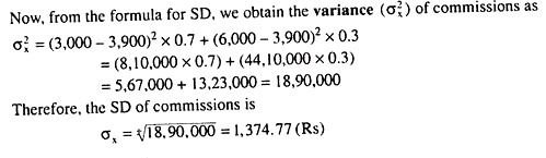
In order to understand the above formula for SD we may take help of the following example. Let us suppose that the probabilities of getting commissions of Rs 3,000 and Rs 6,000 from a particular job are 0.7 and 0.3 respectively.

In this case, the SD of commission (variable X) may be obtained in the following way:

Here E(X) = 0.7 x 3000 + 0.3 x 6000 = 2,100+ 1,800 = 3,900 (Rs)