Support and Stabilisation of Commodity Prices | UNCTAD | Economics

In this article we will discuss about the support and stabilisation of commodity prices by UNCTAD.

In order to help improve the terms of trade of primary products, UNCTAD-IV dwelt upon the issue of stabilisation of international commodity prices and the creation of an integrated programme for commodities. The prices of primary products fluctuate widely in the short run and have a long term tendency to move downwards relative to the prices of manufactured products. The LDC’s are thus faced with the instability of export earnings.

Such instability gives rise to several problems including the difficulty in planning development and inhibition of development process. The stabilisation of commodity prices can enable the LDC’s to get over those problems. In this connection, it should be noted that stabilising prices is not the same thing as stabilising export earnings. The stabilising of export earning is not necessarily the same thing as stabilising real income.

It is important to identify what form of price variability should be brought under control. The short term variability in prices seems to result from random shocks in the supply of a commodity such as changes in weather and incidence of disease in an agricultural crop. Medium term variability in prices may be on account of variations in demand caused by trade cycle on the international plane and variations in supply of the type of Cob-web theorem.

The long run variability in the prices of primary products may arise from long term shifts in supply and/or demand functions. The decline in the demand for a product over time occurs because of the development of new substitutes for a given product and an improvement in technology. There may be an increase in the supply of the product in the long run due to discovery of new sources of supply and improved technology.

Such a distinction is important as the policies that are appropriate for reducing short term variability may be inappropriate for dealing with medium term price variability. Similarly the policies that can control price variability in the medium term are not expedient for controlling price variability in the long run.

Supporting of Prices in the Long Run:

In the long run, the stabilisation of prices has to be considered from the viewpoint of maintaining them in the face of a tendency for them to decline. It is highly unrealistic to attempt to control the long term decline of terms of trade. It is also unrealistic to attempt to maintain stability of prices of primary products over those of industrial products in the long run.

However, one obvious way for manipulating the price of a commodity in a specific way is to form a cartel for regulating the quantity sold of it as is attempted by OPEC. It may be explained through Fig. 32.1 and 32.2.

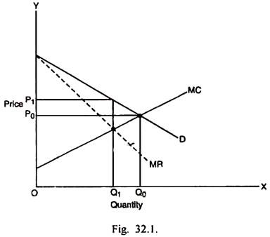
In Fig 32.1, D is the demand curve facing the cartel. It expresses the excess demand for the product in rest of the world over the supply coming from countries outside the cartel. MR curve is the marginal revenue curve facing the cartel. MC is the marginal cost curve related to the members of cartel. It is the horizontal summation of the marginal cost curves of the individual members. In the competitive conditions, there may be P₀ price and Q₀ quantity produced.

The cartel may maximise profits by restricting output to Q₁ and pushing up price to P₁. The success of cartel in this respect requires an agreement on the total exports of the cartel and on the allocation of export quota for the member countries. It also requires that actions of the members should be under supervision because individual member countries can increase their profits by exceeding the export quota allocated to them. Even OPEC has failed to ensure strict compliance of export quota to the member countries.

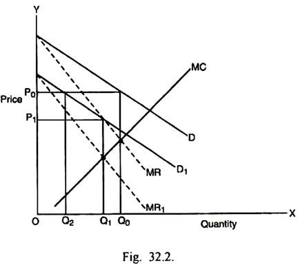
If cartel sets a too high price, it will lead to development of new sources of the product or it will make the importing countries to economise on the use of the product. In either of the two cases, the demand curve faced by the cartel will shift to the left as shown in Fig. 32.2.

Originally the demand curve is D and corresponding marginal revenue curve is MR, the profit maximising output is Q₀ and price is P₀. As the demand curve shifts to the left to D₁, the marginal revenue curve also shift to MR₁ In this situation, the profit maximising output of cartel gets reduced to Q₁ and price falls to P₁.

Profits will also be necessarily lower. Alternatively, if cartel wants to maintain the price at P₀, the output will have to be restricted still further upto Q₂. The fall in profits in this case, will be greater. It is because of such a possibility that Saudi Arabia has often expressed the concern that the high price sought by some OPEC members will produce a severe contraction in demand and consequent steep reduction in the production of oil.

Stabilising Prices in the Medium and Short Run:

In the medium and short run, the more relevant issue is that of stabilising price of primary products rather than supporting them. Mac Bean and Nguyen found that the primary goods were at least 50 percent more variable than the prices of manufactured goods. In some cases, the former were even three times more variables than the latter. They also estimated that export earnings of LDC’s had been about two times more variable than those of the developed industrial countries.

The traditional explanation for this greater instability of prices of primary products emphasised upon low price elasticities of demand and supply for these products. The small changes in quantities supplied, given the low price elasticity of demand, can result in large variation in prices.

The stabilisation of prices, when the price instability is due to variation in supply, is likely to ensure rise in export revenues in the event of large supply level and fall in export revenue in the event of small supply level. It may be explained through Fig. 32.3.

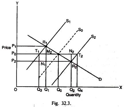
In Fig 32.3, D is the demand curve for the importing country. When supply is low, the supply curve for exporting country is S₁. When the supply is high, the supply curve for the exporting country is S₂. Given D and S₁, the price is high at P₁, the quantity exported is low at Q₁ and export revenue is OQ₁R₁P₁.

Given D and S₂, the price is low at P₂, the quantity exported is high at Q₂, and the export revenue is OQ₂R₂P₂. Whether export revenue is higher or lower in the low supply case depends upon the elasticity of demand curve. If the demand curve is less elastic, OQ₁R₁P₁> OQ₂R₂P₂. On the opposite, if demand curve is more elastic, OQ₁R₁P₁< OQ₂R₂P_2.

Suppose some way is found to stabilize the price at the average level P₀. Given this price, if supply curve is S₁, the quantity exported is Q₃ and the export revenue is OQ₃T₁P₀ which is less than OQ₁R₁P₁. If the supply curve is S₂, at the price P₀, the quantity exported is Q₄ and the export revenue is OQ₄T₂P₀, which is more than OQ₂R₂P₂– By comparing the gain in revenue in high supply period with loss in revenue in low supply period, it may be found that the stabilisation of price at P₀ level will ensure a net gain in export revenue equal to the area N₁R₂N₂M₂.

The stabilisation of prices, however, may cause destabilisation of export revenues in the sense of increasing their variability. In such a situation, the governments which are extremely risk-averse will not be willing to adopt price stabilisation policies particularly when the demand curve for the product is more elastic.

On the other hand, if supply is stabilised at the average level Q₀, there can be the possibility of increase in average export revenue and also the elimination of instability of export revenues. Thus it implies that the policy for stabilising supply is likely to be better than the policy for stabilising price.