Marginal Productivity Theory of Distribution

Marginal Productivity Theory of Distribution: Definitions, Assumptions, Explanation!

The oldest and most significant theory of factor pricing is the marginal productivity theory. It is also known as Micro Theory of Factor Pricing.

It was propounded by the German economist T.H. Von Thunen. But later on many economists like Karl Mcnger, Walras, Wickstcad, Edgeworth and Clark etc. contributed for the development of this theory.

According to this theory, remuneration of cache factor of production tends to be equal to its marginal productivity.

Marginal productivity is the addition that the use of one extra unit of the factor makes to the total production. So long as the marginal cost of a factor is less than the marginal productivity, the entrepreneur will go on employing more and more units of the factors. He will stop giving further employment as soon as the marginal productivity of the factor is equal to the marginal cost of the factors.

Definitions:

“The distribution of income of society is controlled by a natural law, if it worked without friction, would give to every agent of production the amount of wealth which that agent creates.” -J.B. Clark

“The marginal productivity theory contends that in equilibrium each productive agent will be rewarded in accordance with its marginal productivity.” -Mark Blaug

“The marginal productivity theory of income distribution states that in the long run under perfect competition, factors of production would tend to receive a real rate of return which was exactly equal to their marginal productivity.” -Liebhafasky

Assumptions of the Theory:

The main assumptions of the theory are as under:

1. Perfect Competition:

The marginal productivity theory rests upon the fundamental assumption of perfect competition. This is because it cannot take into account unequal bargaining power between the buyers and the sellers.

2. Homogeneous Factors:

This theory assumes that units of a factor of production are homogeneous. This implies that different units of factor of production have the same efficiency. Thus, the productivity of all workers offering the particular type of labour is the same.

3. Rational Behaviour:

The theory assumes that every producer desires to reap maximum profits. This is because the organizer is a rational person and he so combines the different factors of production in such a way that marginal productivity from a unit of money is the same in the case of every factor of production.

4. Perfect Substitutability:

The theory is also based upon the assumption of perfect substitution not only between the different units of the same factor but also between the different units of various factors of production.

5. Perfect Mobility:

The theory assumes that both labour and capital are perfectly mobile between industries and localities. In the absence of this assumption the factor rewards could never tend to be equal as between different regions or employments.

6. Interchangeability:

It implies that all units of a factor are equally efficient and interchangeable. This is because different units of a factor of production are homogeneous, since they are of the same efficiency, they can be employed inter-changeable, and e.g., whether we employ the fourth man or the fifth man, his productivity shall be the same.

7. Perfect Adaptability:

The theory takes for granted that various factors of production are perfectly adaptable as between different occupations.

8. Knowledge about Marginal Productivity:

Both producers and owners of factors of production have means of knowing the value of factor’s marginal product.

9. Full Employment:

It is assumed that various factors of production are fully employed with the exception of those who seek a wage above the value of their marginal product.

10. Law of Variable Proportions:

The law of variable proportions is applicable in the economy.

11. The Amount of Factors of Production should be Capable of being Varied:

It is assumed that the quantity of factors of production can be varied i.e. their units can either be increased or decreased. Then the remuneration of a factor becomes equal to its marginal productivity.

12. The Law of Diminishing Marginal Returns:

It means that as units of a factor of production are increased the marginal productivity goes on diminishing.

13. Long-Run Analysis:

Marginal productivity theory of distribution seeks to explain determination of a factor’s remuneration only in the long period.

Explanation of the Theory:

The marginal productivity theory states that under perfect competition, price of each factor of production will be equal to its marginal productivity. The price of the factor is determined by the industry. The firm will employ that number of a given factor at which price is equal to its marginal productivity. Thus, for industry, it is a theory of factor pricing while for a firm it is a factor demand theory.

Analysis of Marginal Productivity Theory from the Point of View of an Industry:

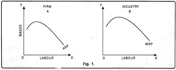
Under the conditions of perfect competition, price of each factor of production is determined by the equality of demand and supply. As the theory assumes that there exists full employment in the economy, therefore, supply of the factor is assumed to be constant. So, factor price is determined by its demand which itself is determined by the marginal productivity. Thus, under such conditions, it becomes essential to throw light on the demand curve or marginal productivity curve of an industry.

As the industry consists of a group of many firms, accordingly, its demand curve can be drawn with the demand curves of all the firms in the industry. Moreover, marginal revenue productivity of a factor constitutes its demand curve. It is only due to this reason that a firm’s demand or labour depends on its marginal revenue productivity. A firm will employ that number of labourers at which their marginal revenue productivity is equal to the prevailing wage rate.

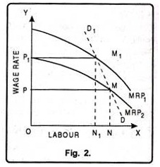
Fig. 2 shows that at wage rate OP₁, the demand for labour is ON₁ and marginal revenue productivity curve is MRP₁. If wage rate falls to OP, firms will increase production by demanding more labour. In such a situation the price of the commodity will fall and marginal revenue productivity curve will also shift to MRP₂.

At OP wages, the demand for labour will increase to ON. DD₁ is the firm’s demand curve for labour. The summation of demand of all the firms shows demand curve of an industry. Since the number of firms is not constant under perfectly competitive market, it is not possible to estimate the summation of demand curves of all firms. However, one thing is certain that is the demand curve of industry also slopes downward from left to right. The point where demand for and supply of a factor are equal will determine the factor price for the industry. This theory assumes the supply of a factor to be fixed.

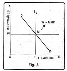
Thus factor price is determined by the demand for factor i.e. factor price will be equal to the marginal revenue productivity. It has been shown by Fig. 3. In the Fig. 3, number of labour has been taken on OX axis whereas wages and MRP have been taken on OY axis. DD₁ is the industry’s demand curve for labour. This is also the Marginal Revenue Productivity curve.

Factor Price (OW) = Marginal Revenue Productivity MRP.

Thus under perfect competition, factor price is determined by the industry and firm demands units of a factor at this price.

Analysis of Marginal Productivity Theory from the Point of View of Firm:

Under perfect competition, number of firms is very large. No single firm can influence the market price of a factor of production. Every firm acts as a price taker and not a price maker. Therefore, it has to accept the prevailing price. No employer would like to pay more than what others are paying. In other words, a firm will employ that number of a factor at which its price is equal to the value of marginal productivity. Therefore, from the point of view of a firm, the theory indicates how many units of a factor it should demand.

It is due to this reason that it is also called Theory of Factor Demand. Other things remaining the same, as more and more labourers are employed by a firm, its marginal physical productivity goes or- diminishing. As price under perfect competition remains constant, so when marginal physical productivity of labour goes on diminishing, marginal revenue productivity will also go on diminishing. Therefore, in order to get the equilibrium position, a firm will employ labourers up to a point where their respective marginal revenue productivity is equal to their wage rate.

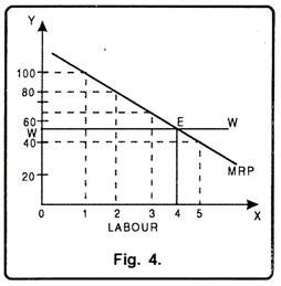
Table 2 indicates that wage rate of labour is Rs. 55 per labourers. Price of the product produced by the labourer is Rs. 5 per unit. Now, when a firm employs one labourer, his marginal physical productivity is 20 units. By multiplying the MPP with price of the product we get marginal revenue productivity. Here, it is Rs. 100 for the first labour. The marginal revenue productivity of second labourer is Rs. 85 and of third labourer it is Rs. 70.

The marginal revenue productivity of fourth labourer is Rs. 55 which is equal to wage rate. The firm will earn maximum profits if it employs up to the fourth labourer. If the firm employs fifth labourer, it will have to suffer losses of Rs. 15. Therefore, to get maximum profits, a firm will employ a factor upto a point where MRP is equal to price.

In Fig. 4 number of labourers has been measured on OX-axis and wage rate on Y-axis. MRP is marginal revenue productivity curve and WW is the wage rate prevailing in the market. Since, under perfect competition wage rate will remain constant that is why WW wage line is parallel to OX-axis.

MRP curve is sloping down-ward. It cuts WW at point E which is the equilibrium wage rate of Rs. 55. At point E, firm will demand only four labourers. Thus, from the above, we can conclude that a factor is demanded up to the limit where its marginal productivity is equal to prevailing price.

 

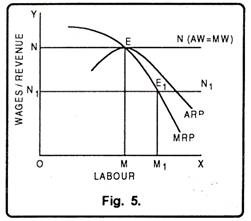
Under perfect competition, in long period in the equilibrium position, not only the marginal wages of a firm are equal to marginal revenue productivity, even the average wages of the firm are equal to average net revenue productivity as has been shown in Fig. 5. The fig. 5 shows that at point ‘E’ marginal wages of labour are equal to marginal revenue productivity and the firm employs OM number of workers. At this point, even the average net revenue productivity is equal to average wages. Thus firm earns only normal profit. If wage line shifts from NN to N[N] then the demand for labour increases from OM to OM₁.

 

Determination of Factor Pricing under Imperfect Competition:

Marginal productivity theory applies to the condition of perfect competition. But in real life we face imperfect competition. Therefore, economists like Robinson, Chamberlin have analyzed factor pricing under imperfect competition. There are various firms under imperfect competition. But here we shall analyze only Monopsony. Under monopsony, there is perfect competition in product market. Consequently MRP is equal to VMP. There is imperfect competition in factor market.

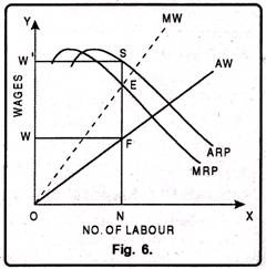
It indicates that there is only one buyer of the factors. Therefore, monopsony refers to a situation of market where only a single firm provides employment to the factors. If the firm demands more factors, factor price will go up and vice-versa. However, the determination of factor price under monopsony can be explained with the help of Fig. 6.

In Fig. 6 number of labourers has been shown on X-axis and wages on Y-axis. MW is marginal wage curve and ARP is the average wage curve. MRP is the marginal revenue productivity curve and AW is the average revenue productivity curve.

In the fig. 6 a monopsony will employ that number of labourers at which their marginal wage is equal to MRP. In the fig. 6 firm is in equilibrium at point E. Here, firm will employ ON labourers and they will be paid wages equal to NF. In this way, ON labourers will get less wages than their MRP i.e. EN. Monopsony firm will have EF profit per labourer which arises due to exploitation of labourers. Total profit SFWW’ is due to exploitation of labour.